MACHINE LEARNING FOR MARKETERS
A Comprehensive Guide to Machine Learning

A Comprehensive Guide to Machine Learning

Diving deeper into the topics surrounding Machine Learning, we’re confronted with a copious amount of jargon. It helps our journey to understand how professionals in the space discuss the topics so that we can become familiar with the terms we’ll run into as we dive deeper into Machine Learning.
Our goal will be providing an understanding of the various topics without getting too deep into the technical details. We know your time is important, so we’re making sure that the time spent learning the language of Machine Learning will pay off as we go down the path of utilization and use cases.
Revisiting Supervised And Unsupervised Machine Learning
We grazed past the concept of supervised and unsupervised learning in Chapter 1; however, these topics are important, and they deserve a more in-depth study.
As previously discussed, supervised Machine Learning involves human interaction elements to manage the Machine Learning process. Supervised Machine Learning makes up most of the Machine Learning in use. The easiest way to understand supervised Machine Learning is to think of it involving an input variable (x) and an output variable (y). You use an algorithm to learn a mapping function that connects the input to the output. In this scenario, humans are providing the input, the desired output, and the algorithm.
Let’s look at supervised learning in terms of two types of problems:
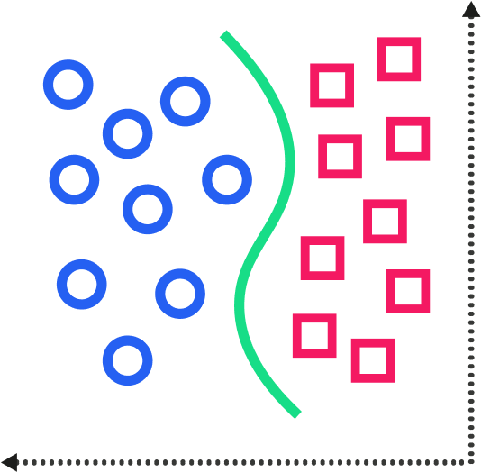
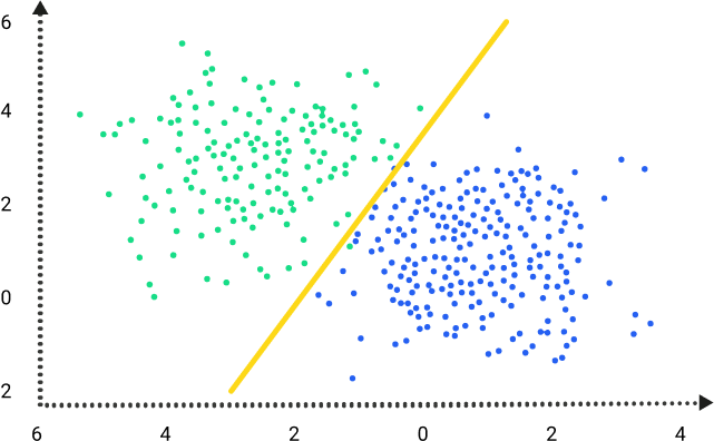
Classification – The output variable of classification problems is categorical, like sex and age group. A common model for these types of problems is Support Vector Machine (SVM). Despite their odd name, The SVM model is a way we describe a linear decision boundary between classes that maximizes the width of the boundary itself.
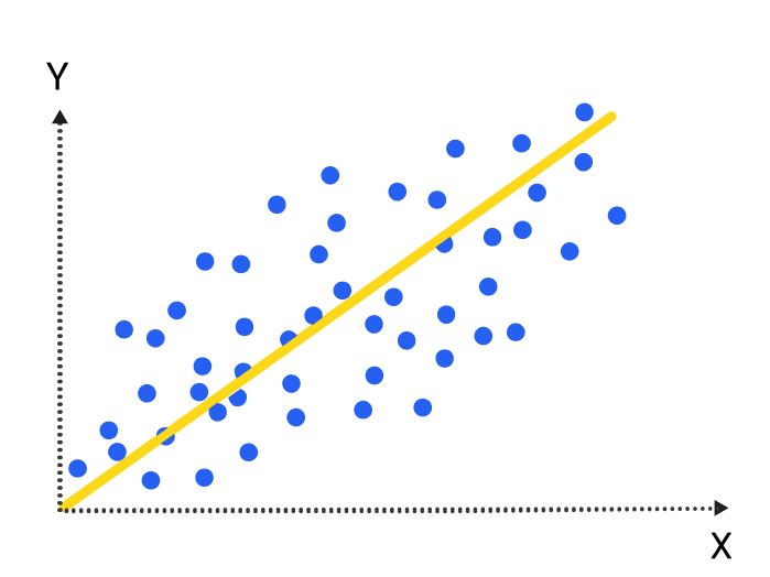
Regression – Regression problems are where the output variables are continuous. A common format of these types of problems are linear progressions. Linear regression models determine the impact of
a number of independent variables on a dependent variable (such
as sales) by seeking a “best fit” that minimizes squared error. Other regression models combine linear models for more complex scenarios.
As opposed to supervised learning, unsupervised learning involves only entering data for (x). In this model, a correct answer doesn’t exist, and a “teacher” is not needed for the “learner.” You’ll find two types of unsupervised Machine Learning: clustering and association.
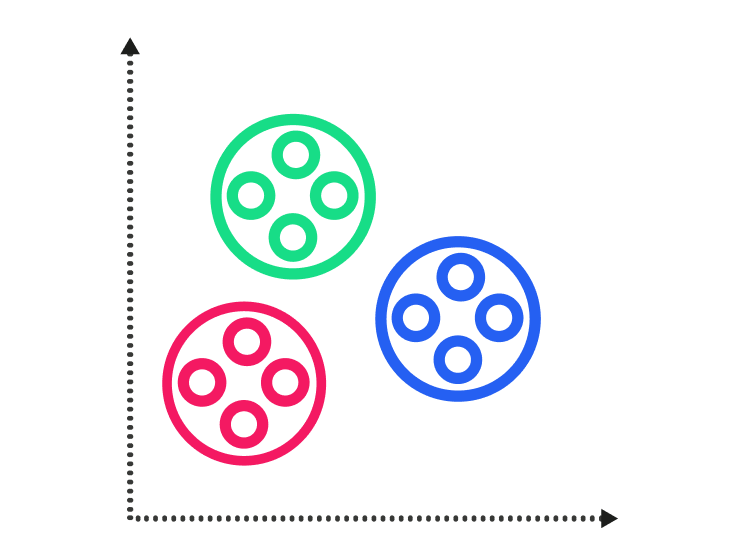
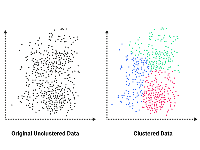
Clustering – This type describes techniques that attempt to divide data into groups clustered close together. An example of clustering is grouping customers by their purchasing behavior.
Association – This type describes techniques that create rules that explore the connections among data. An example is helpful here: We might say that people who buy X product also often buy Y product.
But wait … you’ll also find a third type of Machine Learning technique, semi-supervised Machine Learning. Think of this type as a hybrid between the two previously mentioned models. In most cases, this type of learning happens when you’ve got a large data set for (x), but only some of (y) is definitive and capable of being taught. Semi-supervised Machine Learning can be used with regression and classification models, but you can also use them to create predictions.
A decision tree model builds a series of branches from a root node, splitting nodes into branches based on the “purity” of the resulting branches. You use decision trees to classify instances: One starts at the root of the tree. By taking appropriate branches according to the attribute or question asked at each branch node, one eventually comes to a leaf node. The label on that leaf node is the class for that instance. This modeling is the most intuitive type of modeling. You’ve likely used some version of it in your school or professional life.
Backed-up Error Estimate – In order to prune decision trees and keep the “purity” of each branch of the tree, you must decide whether an estimated error in classification is greater if the branch is present or pruned. A system to measure these issues takes the previously computed estimated errors associated with the branch nodes, multiplies them by the estimated frequencies that the current branch will classify data to each child node, and sums the resulting products. Training data gets used to estimate instances that are classified as belonging to each child node. This sum is the backed-up error estimate for the branch node.
Naive Bayes – Naive Bayes classifiers are based on applying Bayes’ theorem with naive independence assumptions between the features. Bayesian inference focuses on the likelihood that something is true given that something else is true. For example, if you’re given the height and weight of an individual and are asked to determine whether that person is male or female, naive Bayes can help you to make assumptions based on the data.
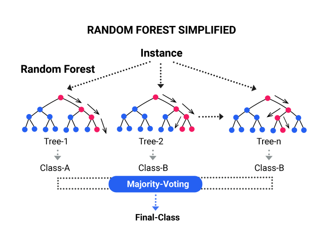
Random Forest – Compared with the decision tree model which relies on a single tree, the random forest model leverages the power of multiple decision trees for prediction. It is what “forest” means. Each decision tree in the andom forest is trained by a random subset of features to generate an output. Finally, the random forest combines the output of each individual decision tree to generate the final output.
As discussed in the previous chapter, reinforced learning is a Machine Learning evolution that involves neural network development. Reinforced learning combines multiple layers of networks into complex models that are useful for building intelligent models.
Neural Networks – This collection of artificial neurons (or Machine Learning and algorithmic layer) gets linked by directed weighted connections. Each neural network layer feeds the next. The neural network levels each have input units clamped to desired values. Clamping – This action takes place when a layer, also called a “neuron,” in a neural network has its value forcibly set and fixed to some externally provided value, otherwise called clamping. Activation Function – This function describes the output behavior of a neuron. Most networks get designed around the weighted sum of the inputs.
Asynchronous vs. Synchronous – Some neural networks have layers of computations that “fire” at the same time, with their nodes sharing a common clock. These networks are synchronous. Other networks have levels that fire at different times. Before you stop us, let’s clarify something for you: We’re not saying that there’s not a pattern to how the levels handle input and output data; we’re only saying that the levels aren’t firing in a precisely timed way.
Dimensionality Reduction – This concept uses linear algebra to find correlations across data sets.
Principal Component Analysis (PCA) – This process identifies uncorrelated variables called principal components from a large set of data. The goal of principal component analysis is to explain the maximum amount of variance with the fewest number of principal components. This process is often used in utilities that work with large data sets. Singular Value Decomposition (SVD) – This technique combines information from several vectors and forms basis vectors that can explain most of the variances in the data.

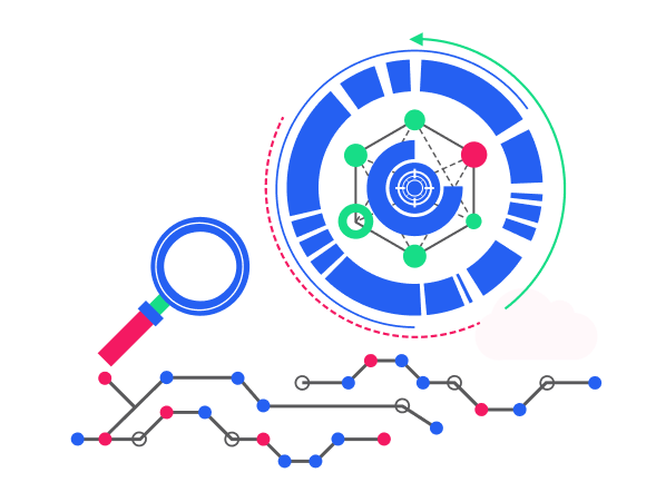
Graph Analysis – This process involves using “edges” connected to other numerical data points to analyze networks. The data points are known as nodes, and the edges are the ways in which they get connected. Facebook’s EdgeRank, which was replaced by a more advanced Machine Learning algorithm, got its name from graph theory.
Similarity Measures – Sometimes known as a similarity function, a similarity measure quantifies the similarity between two objects. Cosine similarity is a commonly used similarity measure. This measurement is used in information retrieval to score the similarity between documents. Clustering uses similarity measures to determine the distance between data points. Shorter distances are equivalent to greater similarity.
![]()
![]()
Diving deeper into the topics surrounding Machine Learning, we’re confronted with a copious amount of jargon. It helps our journey to understand how professionals in the space discuss the topics so that we can become familiar with the terms we’ll run into as we dive deeper into Machine Learning.
Our goal will be providing an understanding of the various topics without getting too deep into the technical details. We know your time is important, so we’re making sure that the time spent learning the language of Machine Learning will pay off as we go down the path of utilization and use cases.
Revisiting Supervised And Unsupervised Machine Learning
We grazed past the concept of supervised and unsupervised learning in Chapter 1; however, these topics are important, and they deserve a more in-depth study.
As previously discussed, supervised Machine Learning involves human interaction elements to manage the Machine Learning process. Supervised Machine Learning makes up most of the Machine Learning in use. The easiest way to understand supervised Machine Learning is to think of it involving an input variable (x) and an output variable (y). You use an algorithm to learn a mapping function that connects the input to the output. In this scenario, humans are providing the input, the desired output, and the algorithm.
Let’s look at supervised learning in terms of two types of problems:
Classification – The output variable of classification problems is categorical, like sex and age group. A common model for these types of problems is Support Vector Machine (SVM). Despite their odd name, The SVM model is a way we describe a linear decision boundary between classes that maximizes the width of the boundary itself.
Regression – Regression problems are where the output variables are continuous. A common format of these types of problems are linear progressions. Linear regression models determine the impact of
a number of independent variables on a dependent variable (such
as sales) by seeking a “best fit” that minimizes squared error. Other regression models combine linear models for more complex scenarios.
As opposed to supervised learning, unsupervised learning involves only entering data for (x). In this model, a correct answer doesn’t exist, and a “teacher” is not needed for the “learner.” You’ll find two types of unsupervised Machine Learning: clustering and association.
Clustering – This type describes techniques that attempt to divide data into groups clustered close together. An example of clustering is grouping customers by their purchasing behavior.
Association – This type describes techniques that create rules that explore the connections among data. An example is helpful here: We might say that people who buy X product also often buy Y product.
But wait … you’ll also find a third type of Machine Learning technique, semi-supervised Machine Learning. Think of this type as a hybrid between the two previously mentioned models. In most cases, this type of learning happens when you’ve got a large data set for (x), but only some of (y) is definitive and capable of being taught. Semi-supervised Machine Learning can be used with regression and classification models, but you can also use them to create predictions.
A decision tree model builds a series of branches from a root node, splitting nodes into branches based on the “purity” of the resulting branches. You use decision trees to classify instances: One starts at the root of the tree. By taking appropriate branches according to the attribute or question asked at each branch node, one eventually comes to a leaf node. The label on that leaf node is the class for that instance. This modeling is the most intuitive type of modeling. You’ve likely used some version of it in your school or professional life.
Backed-up Error Estimate – In order to prune decision trees and keep the “purity” of each branch of the tree, you must decide whether an estimated error in classification is greater if the branch is present or pruned. A system to measure these issues takes the previously computed estimated errors associated with the branch nodes, multiplies them by the estimated frequencies that the current branch will classify data to each child node, and sums the resulting products. Training data gets used to estimate instances that are classified as belonging to each child node. This sum is the backed-up error estimate for the branch node.
Naive Bayes – Naive Bayes classifiers are based on applying Bayes’ theorem with naive independence assumptions between the features. Bayesian inference focuses on the likelihood that something is true given that something else is true. For example, if you’re given the height and weight of an individual and are asked to determine whether that person is male or female, naive Bayes can help you to make assumptions based on the data.
Random Forest – Compared with the decision tree model which relies on a single tree, the random forest model leverages the power of multiple decision trees for prediction. It is what “forest” means. Each decision tree in the andom forest is trained by a random subset of features to generate an output. Finally, the random forest combines the output of each individual decision tree to generate the final output.
As discussed in the previous chapter, reinforced learning is a Machine Learning evolution that involves neural network development. Reinforced learning combines multiple layers of networks into complex models that are useful for building intelligent models.
Neural Networks – This collection of artificial neurons (or Machine Learning and algorithmic layer) gets linked by directed weighted connections. Each neural network layer feeds the next. The neural network levels each have input units clamped to desired values. Clamping – This action takes place when a layer, also called a “neuron,” in a neural network has its value forcibly set and fixed to some externally provided value, otherwise called clamping. Activation Function – This function describes the output behavior of a neuron. Most networks get designed around the weighted sum of the inputs.
Asynchronous vs. Synchronous – Some neural networks have layers of computations that “fire” at the same time, with their nodes sharing a common clock. These networks are synchronous. Other networks have levels that fire at different times. Before you stop us, let’s clarify something for you: We’re not saying that there’s not a pattern to how the levels handle input and output data; we’re only saying that the levels aren’t firing in a precisely timed way.
Dimensionality Reduction – This concept uses linear algebra to find correlations across data sets.
Principal Component Analysis (PCA) – This process identifies uncorrelated variables called principal components from a large set of data. The goal of principal component analysis is to explain the maximum amount of variance with the fewest number of principal components. This process is often used in utilities that work with large data sets. Singular Value Decomposition (SVD) – This technique combines information from several vectors and forms basis vectors that can explain most of the variances in the data.
Graph Analysis – This process involves using “edges” connected to other numerical data points to analyze networks. The data points are known as nodes, and the edges are the ways in which they get connected. Facebook’s EdgeRank, which was replaced by a more advanced Machine Learning algorithm, got its name from graph theory.
Similarity Measures – Sometimes known as a similarity function, a similarity measure quantifies the similarity between two objects. Cosine similarity is a commonly used similarity measure. This measurement is used in information retrieval to score the similarity between documents. Clustering uses similarity measures to determine the distance between data points. Shorter distances are equivalent to greater similarity.
![]()
![]()