Keyword Research, SEO

January 10, 2017

Clustering vs. Classification: How to Speed Up Your Keyword Research

Modern keyword research is far beyond collecting a list of keywords and search volume. Learn how to speed up your keyword research process with our tried and true methods.

Vicky Qian

Modern keyword research is far beyond collecting a list of keywords and search volume. In our previous post “The Persona-driven Keyword Research Process” by our foreseeing founder Michael King, we discussed the importance of mapping keywords to personas and stages in the user journey/need states. However, most marketers who have actually done keyword research are usually haunted by the fact that it takes a large portion of time to marry keywords with personas and need states, especially for large websites with more than 30K keywords. It’s quite a time-consuming process to scan through all these keywords and categorize them with filters and formulas in Excel. This is the time when you need machine learning to quicken the process. Today I am going to talk about how to speed up this modern keyword research with clustering and classification.

Before we get our hands dirty and run models in R and Python, let’s first take a look at the concept of clustering and classification.

Unsupervised vs. Supervised Learning

In the context of machine learning, clustering belongs to unsupervised learning, which infers a rule to describe hidden patterns in unlabeled data. Specifically, clustering is the process of grouping a set of items in such a way that items in the same group are more similar to each other than those in other groups. In keyword research, we can cluster keywords by topics, personas or need states in the user journey.

On the other hand, classification is a type of supervised learning, which fundamentally infers a function from labeled training data. The labels in the context of keyword research can be topics, personas and need states for keywords. For example, to classify the keywords into different need states, we first need a training set of keywords whose need states are known. With a well-trained classifier, we will be able to predict the need states for new keywords. Feel confused with so many terms? Let me explain through an example:

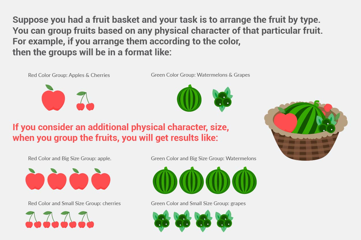
In this case, you didn’t know the rule of grouping fruits before you started, which means no training data and no labels in a machine learning context. This type of learning is known as unsupervised learning and clustering falls into this category.

Now let’s arrange the same type of fruit again. This time you already know from your previous work, the shape of each fruit so it is easy to organize fruits by type (e.g.: arrange apples into the red color and big size group). Here your previous work is your training data and the group of fruits is your labels. This type of learning is known as supervised learning. Classification is one type of supervised learning.

K-Means Clustering

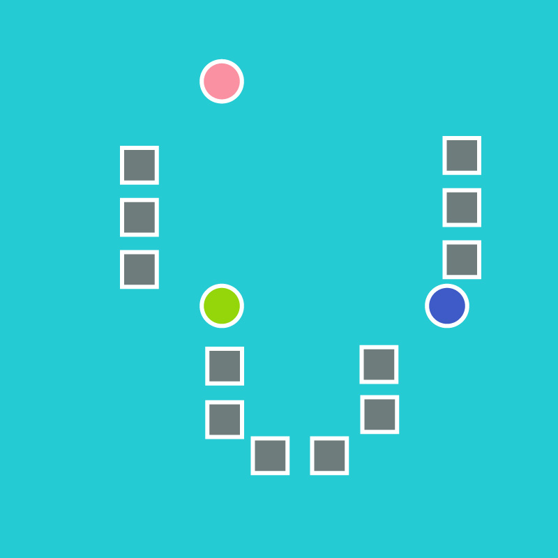
Among all the clustering methods, I will introduce k-means clustering today. K-means is a method of partitioning data into k subsets, where each data element is assigned to the cluster with the nearest mean. The standard algorithm can be demonstrated through the four plots below:

k initial means (in this case k=3) are randomly generated:
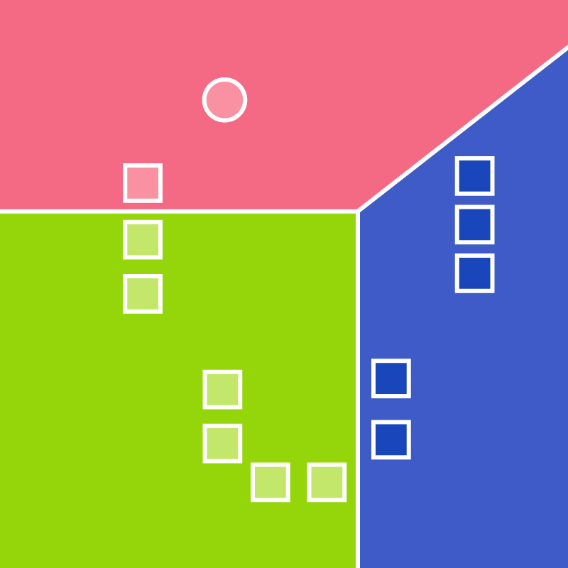
k clusters are created by associating every observation with the nearest mean:
The centroid of each of the k clusters becomes the new mean:
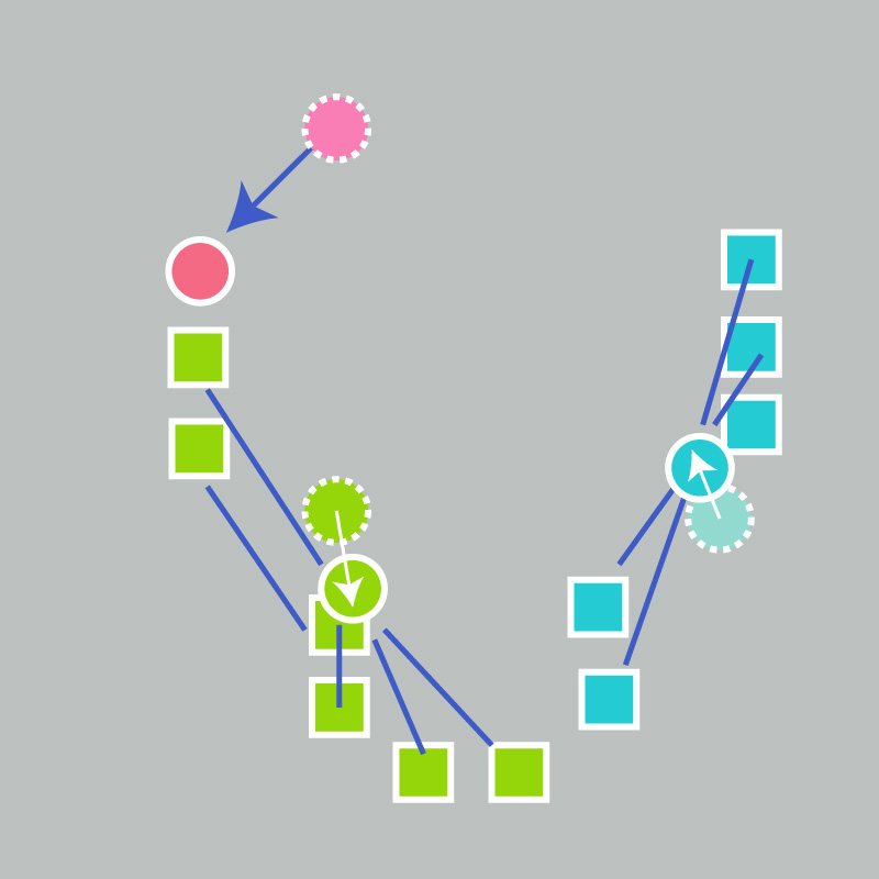
Steps 2 and 3 are repeated until convergence has been reached:

Clustering Keywords Using Google Search Console

Now I am going to experiment with iPullRank’s Search Analytics data from Google Search Console and cluster these keywords into different topics in the following steps:

STEP 1: Preprocess keywords and convert text to numeric data

When preprocessing the data, I only keep the stem of the keywords, remove stop words and punctuation, and set the minimum number of characters to 1. To get a broad idea about the overall search terms, I retrieved the terms with a minimum occurrence frequency of 10.

After preprocessing the data, we need to do some text-to-numeric transformation of our text data. Luckily, R provides several packages to simplify the process. For example, with the tm package, we are able to create a document-term matrix, where each row is one search term and each column is the number of times a single word is contained within that search term.

Detailed code and methodology can be found on Randy Zwitch’s blog: “Clustering Search Keywords Using K-Means Clustering”.

STEP 2: Determine the number of clusters

Once we have the document to term matrix, we can very quickly run the existing package in R. Before we start, we must choose k: the number of clusters expected from the dataset. We could scan through all the keywords and guess how many topics are among the keywords. Or we can use a more automated approach to pick k, which is called Elbow method.

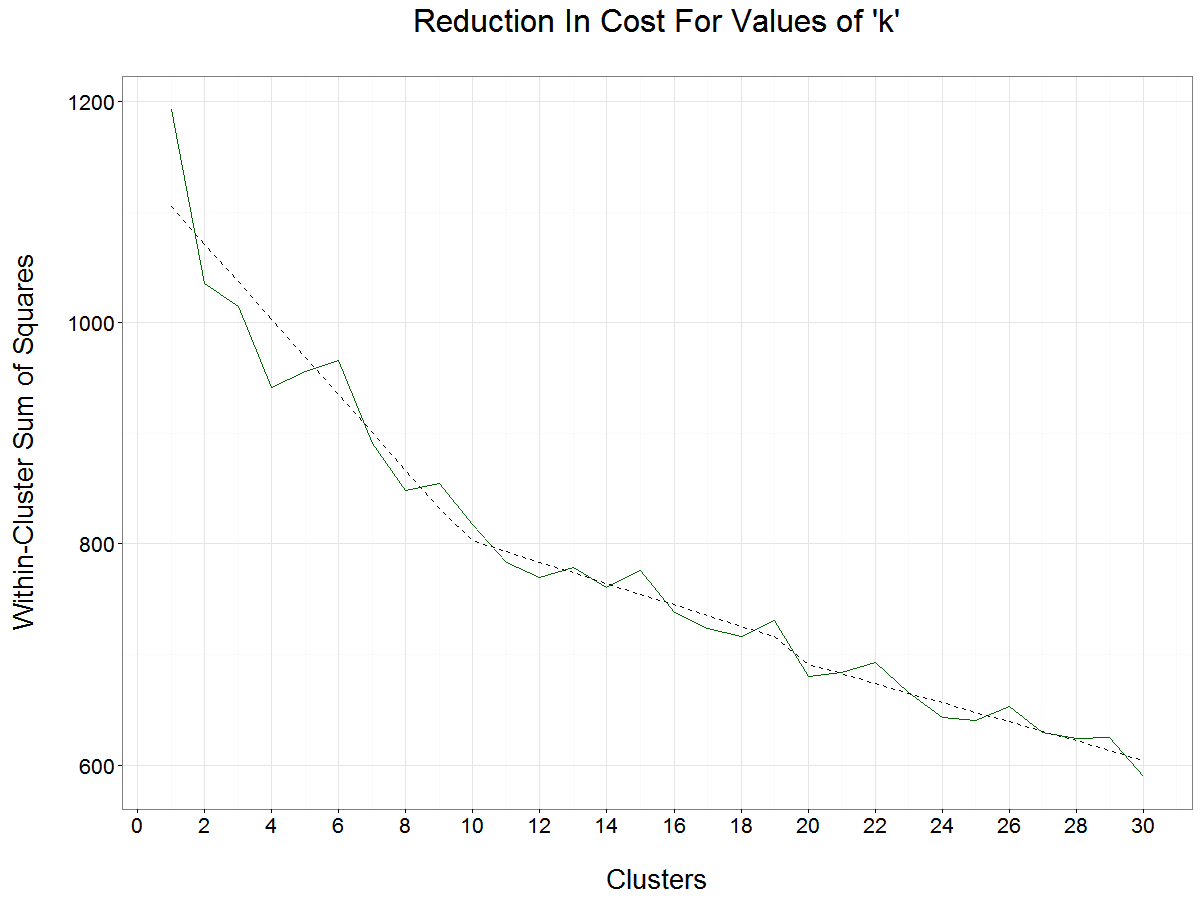
We can calculate the total within-cluster sum of squares for every selection of k, which is a cost function that measures the homogeneity within the same cluster. Intuitively, the more clusters we have, the less within-cluster sum of squares we will get. In one extreme situation where each keyword forms a cluster, the within-cluster sum of squares will reach zero. We need to look for breakpoints where adding another cluster doesn’t give much better modeling of the data.

To illustrate this, I plotted the within-cluster sum of squares for k up to 30. We can see that within-cluster sum of squares continues to drop for k is less than 4, and slightly increases at 5 and 6. The slope of the cost function gets flatter at 10 clusters. This means that as we add clusters above 10 (or 20), each additional cluster becomes less effective at reducing variance. Considering the number of keywords we have (409 in total), 4 is an optimal number of clusters, as 10 would be too granular for a small set of keywords.

Run the model when k=4, and get the most frequent words within each cluster:

As I only kept the stem of words, each word was reduced to a root form, e.g. ‘science’ was reduced to ‘scienc’, ‘blogs’ to ‘blog’, ‘google’ to ‘googl’, etc. It’s not hard to notice that there are some overlapping words between different clusters. For example, ‘googl’ is in cluster 2 and 4, ‘market’ is in cluster 1 and 3. To understand why this happened, I retrieved all the search terms within different clusters. In cluster 2, most search terms that contain ‘googl’ are about Google Tag Manager, while search terms in cluster 4 are related to Googlebot. Similarly, search terms that contain ‘market’ in cluster 1 are mainly about digital marketing/digital marketing analyst content, such as ‘digital marketing analyst’. For cluster 3, a small number of search terms that contain ‘market’ are usually associated with iPullRank, such as ‘mike king marketing’. It’s common that search terms containing one or more same words belong to different topic groups because of the complexity of natural language. A quick scan through all the keywords in different clusters, I concluded that the major topics respectively for clusters 1, 2, 3, and 4 are digital marketing and related content, iPullRank, and Mike King, Googlebot. The process of deciding on main topics with clustering requires some human judgment. This is one of the drawbacks of clustering.

Clustering, in this case, mainly serves the purpose of discovering underlying topics and partitioning search terms into different groups. This process works better for the exploratory scenario where topics are unknown. However, with known topics or labels that you want to categorize the keywords into, classification is a better choice. Classification has a substantial advantage over clustering because classification allows us to take advantage of our own knowledge about the problem we are trying to solve. Instead of just letting the algorithm work out for itself what the classes should be, we can tell it what we know about the classes such as how many there are and what examples of each one look like. The classification algorithm’s job is then to find the features in the examples that are most useful in predicting the classes.

Mapping Keywords to Need States

Another important process in keyword research is mapping the keywords with the user’s need state. For this task, classification is the right tool in the machine learning toolbox. I will discuss two commonly used machine learning models in text classification: multinomial Naive Bayes classifier and Support vector machine (SVM).

Multinomial Naive Bayes classifier is a probabilistic classifier applying Bayes’ theorem for multinomially distributed data, which assumes that the value of a particular feature is independent of the value of any other feature, given the class variable. For example, a fruit may be considered to be an apple if it is red, round, and about 10 cm in diameter. A naive Bayes classifier considers each of these features to contribute independently to the probability that this fruit is an apple, regardless of any possible correlations between the color, roundness, and diameter features.

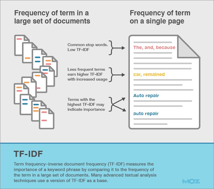
The data are typically represented as word vector counts, however, this will lead to a problem: if a given class and feature value never occur together in the training data, then the frequency-based probability estimate will be zero (according to Bayes’ theorem). This is problematic because it will wipe out all information in the other probabilities when they are multiplied. To alleviate those problems, I include the use of (“Term Frequency-Inverse Document Frequency”) weights instead of raw term frequencies and document length normalization. Tf- idf as a weighting factor is intended to reflect how important a word is to a document in a collection or corpus. Another advantage of using tf-idf is that it helps to adjust for the fact that some words appear more frequently in general. It downscales weights for words that occur in many documents in the corpus and are therefore less informative than those that occur only in a smaller portion of the corpus. For example, if we compare the phrases “car” to “auto repair” in Google’s Ngram viewer, we find that “auto repair” is rarer than “car”. That means the search term “auto repair” has a higher weight than “car” using td-idf because of scarcity.

Source: Moz

Now let’s get to the topic and classify the keywords into different need states using the scikit-learn package in Python (detailed examples and code can be found here). To train the multinomial Naive Bayes classifier, I first need to get a training dataset containing the keywords and labels, which are the need states keywords are classified to (i.e. awareness, interest, and action in our case). The sample training dataset is in the following format:

After training the classifier, the test result shows that: multinomial Naive Bayes classifier reaches 92.4% overall accuracy. To have a better understanding of the classifier performance, I further inspect the results with a confusion matrix:

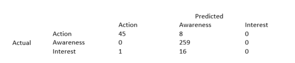
In this confusion matrix, of the 53 actual action keywords, the classifier predicted that 45 were in the action state and of the 259 actual awareness keywords, it predicted that all were in the awareness state. Similarly, among the 17 actual interest keywords, none of them were classified correctly as interest. The classifier tends to classify keywords into action and awareness states and none of the test keywords is classified as interest. This is because the multinomial Naive Bayes classifier is probability-based our dataset contains few keywords in interest state and skews towards the awareness state. It’s unlikely to have keywords classified as interest in test data given the rules learned from the training dataset. As an improvement, we can include more interest keywords in the training dataset in the future. To understand the classifier better, I retrieve the top ten most important features for each category.

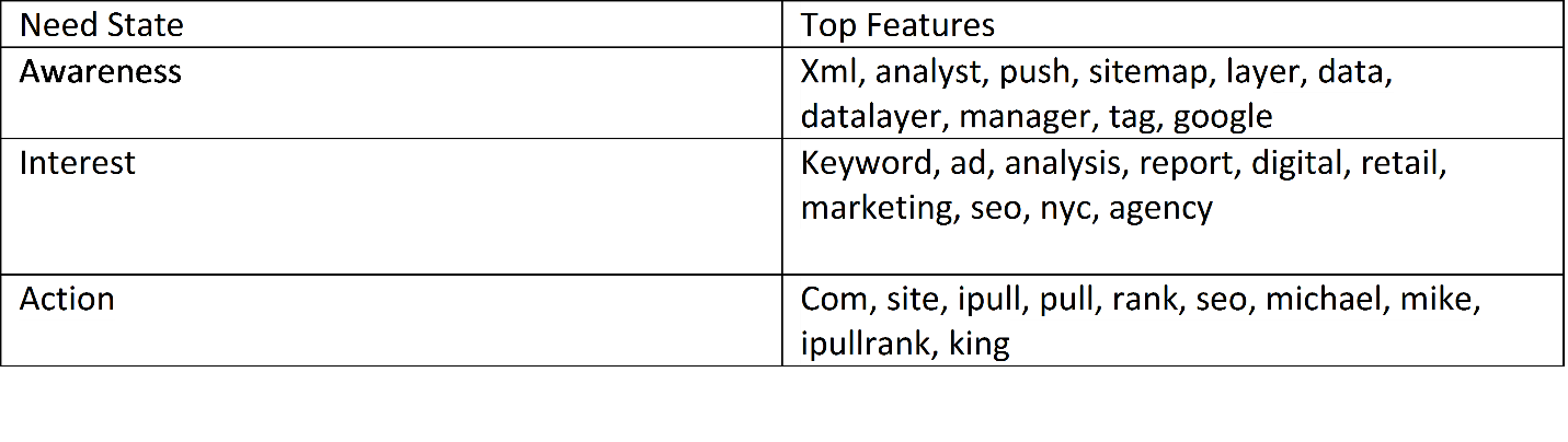
In the awareness state, visitors are driven to the site by high-value content. In interest state, top features include digital, marketing, SEO, NYC, and agency, which indicates that users are searching for digital marketing agencies. In the action state, the key differentiators are the branded terms including Mike King, iPullRank, etc.

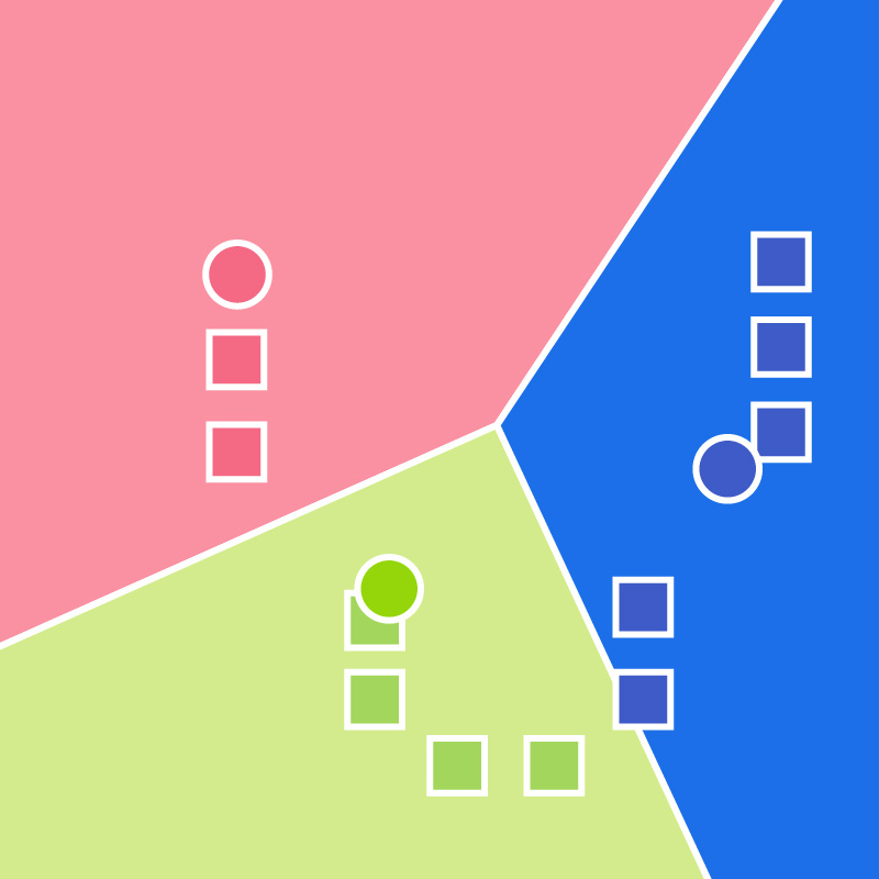
Support vector machine (SVM) is a non-probabilistic classifier that illustrates examples of the separate categories divided by a clear gap that is as wide as possible. The support vector machine for the linearly separable case can be illustrated in the following figure:

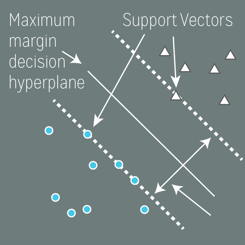
There are lots of possible linear separators for two-class training sets. Intuitively, a decision boundary drawn in the middle of the two classes seems better than the one that is very close to examples of one or both classes. The SVM, in particular, defines the criterion for a decision surface that is maximally far away from any data point. This distance from the decision surface to the closest data point determines the margin of the classifier. This method of construction means that the decision function for an SVM is fully specified by a small subset of the data which defines the position of the separator. These points are referred to as the support vectors. The figure above shows the margin and support vectors for a linear separable problem.

Now let’s get back to our classification problem using SVM in Python (sample code). To make SVM comparable to Multinomial Naive Bayes, I use the same training dataset for both classifiers. SVM hits 93.6% overall accuracy (vs. 92.4% for Multinomial Naive Bayes classifier). Similarly, I retrieve the confusion matrix.

Confusion matrix for SVM:

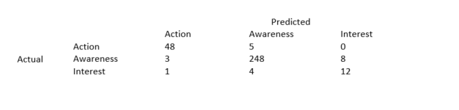
Compare to Multinomial Naive Bayes classifier, SVM has better performance in terms of overall accuracy for this dataset, especially when classifying actual interest keywords. 12 out 17 actual interest keywords are correctly classified as interest.

SVM with the proper choice of kernel has the capability of learning non-linear trends, which is one of the biggest advantages over probability-based Multinomial Naive Bayes. Naive Bayes treats features as independent, whereas SVM looks at the interactions between them to a certain degree, as long as you’re using a non-linear kernel (Gaussian, rbf, poly etc.). There is no single answer about which is the best classification method for a given dataset. But in the end, it all comes down to the tradeoff between bias and variance. An ideal model should be able to accurately captures the regularities in its training data, and also generalizes well to unseen data. Unfortunately, it is typically impossible to do both simultaneously. Learning methods with high variance are usually more complex and represent the training set well, but are at risk of overfitting to noisy or unrepresentative training data. In contrast, high-bias algorithms tend to be relatively simple, but may underfit their training data, failing to capture important regularities. As such, a tradeoff needs to be made when selecting models of different flexibility and complexity.

In short, this blog provides two practical machine learning techniques to speed up keyword research. Clustering is a primary go-to for exploratory analysis, particularly when you have no idea about the topics of the search terms. For a more complicated scenario like classifying search queries to the known topic groups or need states, classifier, either probabilistic or non-probabilistic, undoubtedly is a better choice. Here are some useful resources where you can learn more about the concepts I mentioned in the blog: