
Many users have heard of the VLOOKUP function for Excel but aren’t clear about what it does. Others might just need a refresher. Either way, we’re here to answer any questions you might have.
VLOOKUP refers to the vertical lookup of values in Excel. This function is most useful to reference a value in the corresponding rows of a column. When you have an extensive series of data such as countless rows of user ids and you need to find values associated with them, VLOOKUP is your friend. This function is one of the most used and can simplify wrangling data.
What does VLOOKUP do?
VLOOKUP is a built-in function on Excel (or Google Sheets) designed to work with data that has been organized into columns. Provided a specified value, VLOOKUP essentially “looks up” a value from one column and responds with the corresponding value from another column. This function simplifies the referencing of data and honestly makes my life easier as a Data Analyst.
VLOOKUP will “look up” one value in the column of a table and return its corresponding value from another column where the lookup value is matched.
The syntax is:
=VLOOKUP(lookup_value, table_array, col_index_num, [range_lookup])
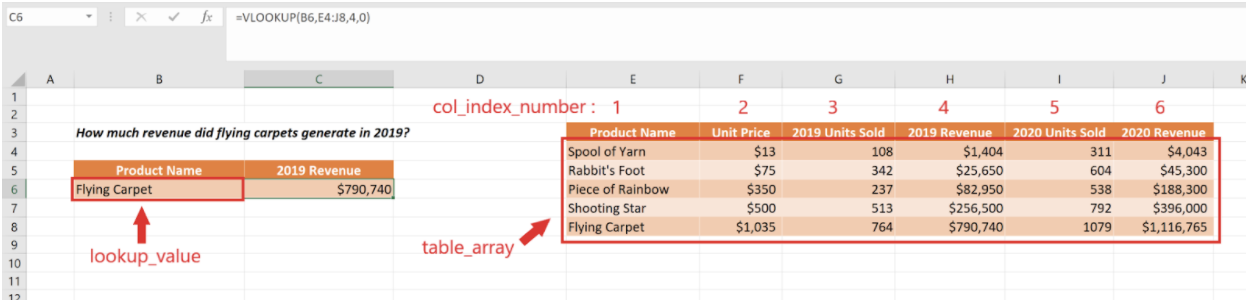
- Lookup_value is the value you want to look up and that will be used to match data. This is usually an identifier (an ID of some kind). The value must exist in the worksheet you reference.
- Table_array is the table from which you want to retrieve data.
- Remember that the lookup value should always be the first column of the range you are looking for your value in. For example, if your lookup value is found in cell B4 of your worksheet, your table array/ range should begin with column letter B.
- Col_index_num is the number of the column from the left side of
the table_array from which you want to retrieve data.- If your range is B2:G24, your first column would be B and C would be your second column. If you are looking for data in column E, your column index number would be “4”.
- Range_lookup defines whether or not the lookup_value is an approximate match or an exact match of the value you are comparing it to in the left-most column of the table_array.
- TRUE: Approximate match is needed.
- FALSE: An exact match is required.
- Instead of typing out “true” or “false”, I personally prefer using “1” for a true/approximate match or “0” for a false/exact match.
NOTE: * True is selected by default. This option is only useful for numeric tables, sorted in ascending order.
In other words,
=VLOOKUP(lookup value, range containing the lookup value, the column number in the range containing the value you’re looking for, approximate match (TRUE / 1) or Exact match (FALSE / 0)).
How do I reference data from another worksheet or workbook?
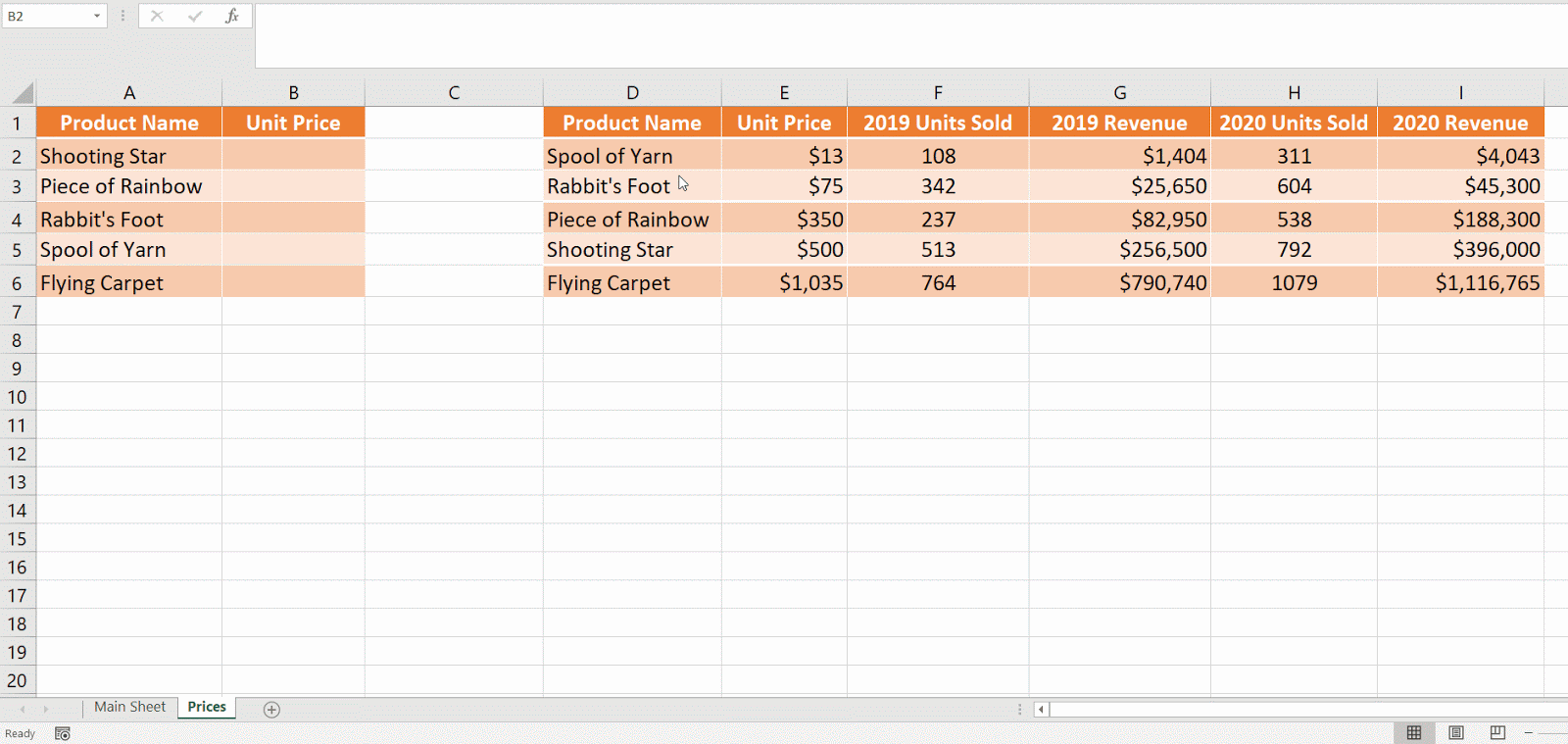
Many times, the data you are looking to reference lives elsewhere and might be buried among other data points. To find your value, simply reference its location in the formula.
The only difference in referencing data on a separate sheet is that the exact name of the sheet followed by “!” must be included in the function as demonstrated above.
=vlookup(A2, Prices!A2:B6, 2, 0)
To reference data in a different workbook, you must also follow certain rules of the function.
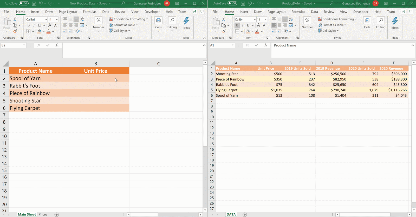
=vlookup(A2, [ProductDATA.xlsx]DATA!$A$2:$F$6,2,0)
[ExactWorkbookName.xlsx]WorksheetName!
NOTE: *The reference used in the above argument is an absolute reference, meaning that the column and row references are prefixed with dollar signs ($). This ensures that your range doesn’t shift when you copy your formula to other cells. You can manually place these before the cell letter to lock the column and after the cell letter to lock the row. You can also press F4 to lock the cell values in your function.
When should VLOOKUP be used?
Keep in mind that VLOOKUP can only be used to reference data on the leftmost column of your range. Therefore, VLOOKUP can only pull data to the right of the reference column. This shouldn’t be too much of a limitation, as most columns will already be to the right.
VLOOKUP is also a vertical-based function and will reference data fixed into columns and look from top to bottom. Another key point to note is that VLOOKUP can only look up values based on a single criteria. For example, if you are looking to reference the first and last names of a customer or employee, but their names are separated into different columns, you must first concatenate first and last names into a single column that can then be referenced by VLOOKUP.
When working with what might seem like endless rows and columns and you need to perform quick matches of data that is not left-based, INDEX-MATCH is generally preferred. The INDEX function will return the value from a specific position in an array and MATCH will return the position of the value you are looking for. Together, they are flexible and extremely useful for extracting data from tables or ranges. All-in-all, INDEX-MATCH is not left-based and allows you to be more flexible with referencing values.
What are the limitations of VLOOKUP?
VLOOKUP is great for “looking up” data, but it does have two significant limitations:
- It’s unidirectional, meaning it must work with indexes fixed to the left side of the work area and will return an error or will be unable to reference the appropriate values.
- Because VLOOKUP references a col_index, it’s unable to dynamically update whenever you insert new columns to the table_array.
- To increase your flexibility with the VLOOKUP function, you can name your ranges.
What is the difference between VLOOKUP and LOOKUP?
The main difference between VLOOKUP and LOOKUP is that VLOOKUP will take the leftmost column and find corresponding values in the column you specify. LOOKUP, on the other hand, will look at adjacent rows and columns to find your value, similar to the functions of VLOOKUP for vertical lookups and HLOOKUP for horizontal lookups. LOOKUP can be considered the old-school function to look up values in Excel and does have limitations. When using it, your data must be sorted in ascending order or it will automatically return the closest match if it doesn’t find the value you are referencing. For this reason, both VLOOKUP and HLOOKUP will best suit you when looking for exact matches.
While being one of Excel’s simpler functions, VLOOKUP is one everyone who works with spreadsheets should know. Excel has a multitude of functions that make working with large datasets more manageable. What are some other functions that you’ve found useful working within Excel or Google Sheets?
Let us know in the comments below. Be sure to check out our Blog for more resources and sign up for our newsletter.