Since learning of the importance and magnitude of vector embeddings, I have been proposing that a link index should vectorize the web and make those representations of pages available to SEOs. Fundamentally, with the further integration of machine learning in Google’s ranking systems, vector embeddings are even more important to what we do than an understanding of the link graph. Currently, only search engines and large language modelers have this data at scale. I believe every SEO tool should be providing this data about pages and keywords.
Google has been leveraging vector embeddings to understand the semantics of the web since the introduction of Word2Vec in 2013 (here’s a simpler explanation) through the update we knew as Hummingbird, but the SEO software industry has continued to operate predominantly on the lexical model of natural language understanding. Lesser known tools like InLinks, WordLift, MarketMuse, MarketBrew and the various keyword clustering tools have all done things with this technology, but the popular SEO tools have not surfaced many semantic features.
To some degree this showcases the gap between modern information retrieval and search engine optimization as industries. The common (simplified) understanding of Google in our space is that their systems simply crawl pages, break the content into its lexical components, counts the presence, prominence, and distribution of words, reviews linking relationships, ranks pages by expanding queries and breaking them into n-grams. Once it retrieves posting lists based on the n-grams, it intersects the results, scores that intersected list, sorts by the score and presents the rankings. Then it reinforces what ranks based on user signals. Structurally, the model architecture looks like this:
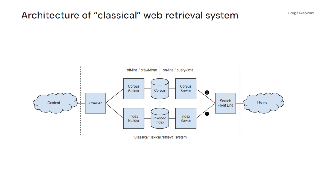
That model is not wrong per se, because Google still does these things. It’s just not at all indicative of the state of the art with which Google Search operates because it does so much more.
Distinguished Google Researcher, Marc Najork, in his Generative Information Retrieval presentation (where the above image comes from) discussed how the state of the art has evolved to fusion-based approaches that are a hybrid between lexical and semantic models. Citing his Google Research team’s own 2020 paper Leveraging Semantic and Lexical Matching to Improve the Recall of Document Retrieval Systems: A Hybrid Approach where they showcase open source libraries to implement and examine the viability of the method. They combine BM25 (the lexical retrieval model SEO effectively still operates on) with Google’s SCaNN package for vector search with BERT for dense vector embeddings and combine and re-rank the results with a method called RM3.
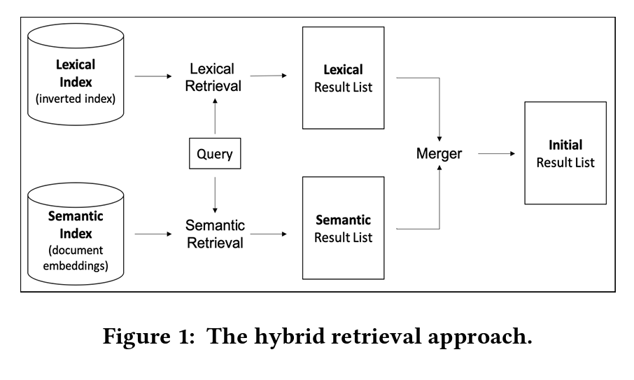
One of the key differences in the models is the advent of nearest neighbor searching with dense vectors. This is why rankings often no longer behave the way we anticipate. Semantic matching, and Google’s specific improvements on it “neural matching,” is often a “fuzzier” understanding of relevance when you’re used to seeing the explicit presence of words in page titles, h1 tags, and distributed across body text and more links with targeted anchor text.
In fact, our mental model of how Google works is quite out of date. Based on what Najork presents in his deck, it looks a lot more like this:
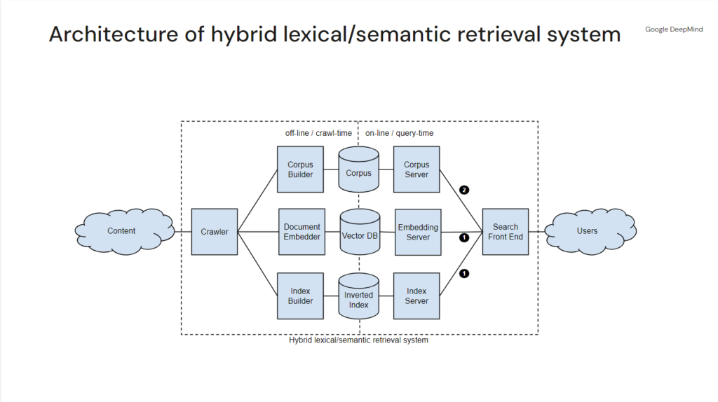
As natural language processing technology has yielded denser embeddings (as compared to the sparse embeddings featured in approaches like TF-IDF), Google has improved its ability to capture and associate information on a passage, page, site, and author level. Google moved on a long time ago, but with the rapid advancements in vector embeddings we can catch up.
What are Vector Embeddings?
As I explained in my “Relevance is not Qualitative Measure for Search Engines” piece, the vector space model is what powers the understanding of relevance between queries and documents. Vector embeddings are used to represent the query and the documents in that model.
I explained this in that post, but in the spirit of saving you a click and improving the relevance for this post, vector embeddings are a powerful technique in natural language processing (NLP) that represent words, phrases, or documents by plotting them as coordinates in multi-dimensional space. These vectors capture the semantic meaning and relationships between words, allowing machines to understand the nuances of language.
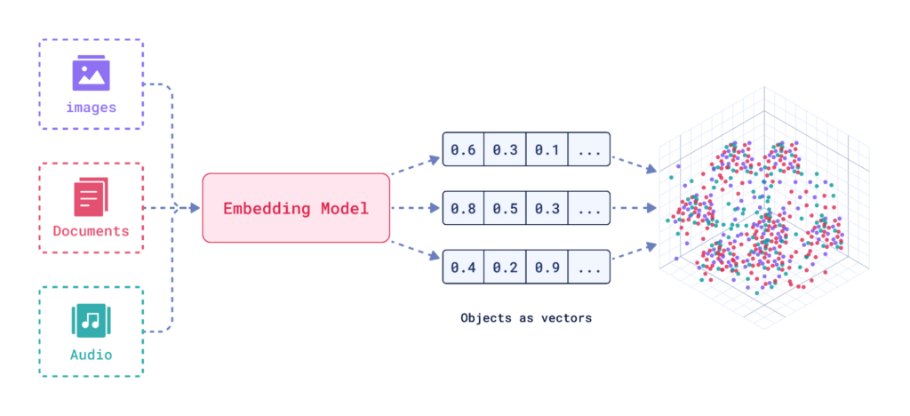
While TF-IDF and its variants yielded simplified word vectors that indicated the presence of words based on a given page’s vocabulary, the history of modern vector embeddings goes back a little over a decade ago. Seminal works like the aforementioned word2vec were introduced in 2013 and capabilities have rapidly improved since the advent of Google’s Transformer. These models learned word relationships by analyzing large text corpora, positioning similar words close together in the vector space. Transformer improved upon a concept called Attention wherein the language model developed the ability to also understand context and polysemy. So when I have the sentence “She bats her eyelashes flirtatiously at her date across the table” and the sentence “At dusk, bats emerged from the cave, flitting about in search of insects,” modern language models can now understand that the second usage of the word “bats” means the noun representing the animal while the first usage of the word “bats” is the verb representing the physical action.
Dense vector embeddings revolutionized search by improving upon semantic search (or vector search), which goes beyond keyword matching to understand the intent behind a query and the meaning of the documents being considered. Search engines can now identify synonyms and related concepts, leading to more relevant and accurate results. When we say we’ve moved form keywords to concepts this is what we’re talking about. Information Retrieval is no longer solely reliant on the presence of specific words, a concept can be represented and measured.
Further still, vectors allow Google to effectively model representations of queries, entities, individual sentences, authors, websites, and use those representations to fulfill the ideas behind E-E-A-T.
State-of-the-art vector embeddings are trained on massive datasets and incorporate contextual information to capture complex relationships between words. This ongoing development continues to improve the accuracy and efficiency of search algorithms.
Enter Screaming Frog SEO Spider’s Custom JavaScript
Screaming Frog SEO Spider has been nudging the SEO space forward for over a decade. The team has continued to innovate in ways that the industry needs, and the SaaS tools are too slow to do. Being in the cloud has its advantages for scalability and speed, but there is nothing any of those tools can do that SFSS can’t, and plenty that it can do that those other tools won’t. When the SF team launches cutting edge features other tools should consider altering their roadmap.
Version 20 is no different. What’s great for my cause is that it seems they are in agreement that someone should help us vectorize the web.
Their new Custom JavaScript functionality allows users to run bespoke JS functions on pages as the spider crawls them. You can now do customized analysis and make calls to third party sources to enhance your crawl data.
While a lot of SEOs are going to use this upgrade to turn SFSS into Scrapebox, one of the operations that comes with the tool is code to generate vector embeddings from OpenAI as you crawl. This is specifically what is going to help you make the upgrade from lexical analysis to semantic.
JavaScript Functions in Screaming Frog
I was going to explain the different functions for accessing things in SFSS, but instead I made you a custom GPT called Kermit with the documentation to help you write your code. Thank me later.
The main functional capabilities to know are that you can:
- run actions on the page
- Run extractions from the page
- save files based on either
- load external scripts
- run multiple operations
- perform operations from the Chrome Utilities API
Unless you’re a JavaScript wizard, I recommend leaning heavily on the custom GPT to get yourself started. I also recommend contributing what you build to this public repository of SFSS custom JS scripts.
How to Vectorize a Site with Screaming Frog SEO Spider
If you’ve used custom extractions in SFSS before, the new Custom JS extraction functionality is an expansion of that. You can define what you want to execute at runtime and store it in unique columns. To get you started, the SF team has prepared a series of templates, including one for capturing embeddings from OpenAI as you crawl. Here’s how you do it:
- In the Crawl Config select Custom > Custom JavaScript
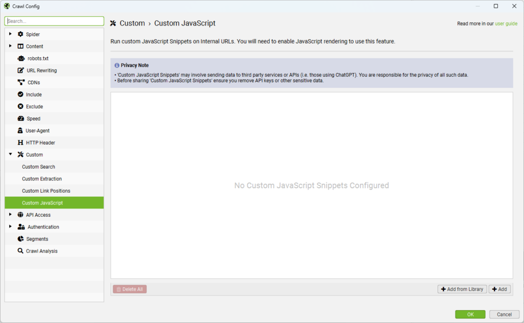
This brings you to a dialog box where you can add and test your custom JS code. Click Add from Library to get the party started.
- Select the ChatGPT extract embeddings from page content
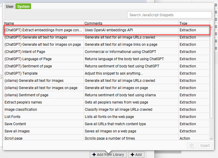
In the system tab you’ll find a series of custom extractions and actions. There are things that can be pulled without external functionality as well as things that can use ChatGPT’s API or a local LLM via ollama. For our purposes, you’ll want the “(ChatGPT) Extract embeddings from page content” function.
- Enter your OpenAI API key.
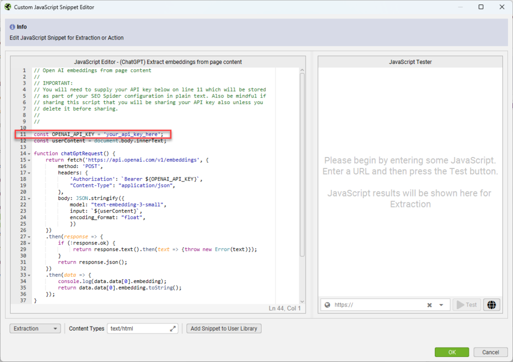
Once you’ve selected the extraction, you’ll need to configure the code by adding your OpenAI API key. You can test it on the right by adding a URL and clicking test. What you’ll get back is a series of decimal numbers. These are your embeddings.
- Configure your crawl as you normally would and make sure to enable JavaScript rendering and that crawling external links is enabled. Then let it run as normal.
When you get your data back your Custom JavaScript tab will look like this:

By default, the embeddings will only be computed on pages that are of text/html type, but embeddings can be multimodal, so if you wanted to compute them on images you could. For that you’d have to adjust the Content Types that the JS fires on and pass the images as bytes.
Do I Have to Use OpenAI?
No, you don’t. In fact, according to the HuggingFace Massive Text Embedding Benchmark (MTEB) Leaderboard, they are not considered state of the art at this point. Google’s text-embedding-preview-0409 embeddings model is smaller with lower dimensionality and outperforms OpenAI’s text-embedding-3-large embeddings model in all tasks.
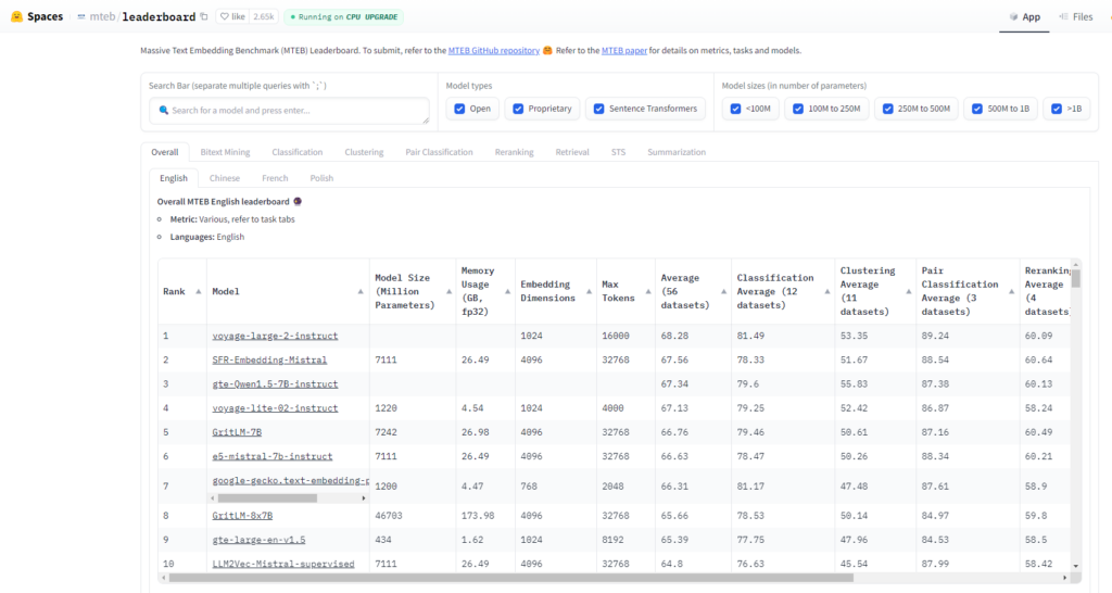
text-embedding-preview-0409 is $0.000025 / 1K tokens. If you did 100 million tokens (or the equivalent of two thousand novels not written by Stephen King), you’re spending $2 with OpenAI and $2.50 with Google. However, if you do batch requests to Google, the pricing is exactly the same. Although, I wonder if this will change based on announcements at the upcoming Google I/O conference.Accounting for Token Limits
The length of your content is also a factor since Google only accepts 3,071 input tokens, whereas OpenAI accepts 8,191. If your content is too long, you’ll get an error message that looks like this:
Error: {
  "error": {
    "message": "This model's maximum context length is 8192 tokens, however you requested 11738 tokens (11738 in your prompt; 0 for the completion). Please reduce your prompt; or completion length.",
    "type": "invalid_request_error",
    "param": null,
    "code": null
  }
}
In these cases you’d have to chunk the content and manage the embeddings into a single set for our use cases. It’s common practice to average the embeddings from the chunks into a single set of embeddings as follows:
const OPENAI_API_KEY = 'your_api_key_here';
const userContent = document.body.innerText;

function chatGptRequest() {
    if (new TextEncoder().encode(userContent).length > 8191) { // Checking byte length approximation for tokens
        // Function to break the string into chunks
        function chunkString(str, size) {
            const numChunks = Math.ceil(str.length / size);
            const chunks = new Array(numChunks);

            for (let i = 0, o = 0; i < numChunks; ++i, o += size) {
                chunks[i] = str.substring(o, o + size);
            }
            return chunks;
        }

        // Divide content into manageable chunks
        const chunks = chunkString(userContent, 8191);

        // Function to request batch embeddings for all chunks
        function chatGptBatchRequest(chunks) {
            return fetch('https://api.openai.com/v1/embeddings', {
                method: 'POST',
                headers: {
                    'Authorization': `Bearer ${OPENAI_API_KEY}`,
                    "Content-Type": "application/json",
                },
                body: JSON.stringify({
                    model: "text-embedding-3-small",
                    input: chunks,
                    encoding_format: "float",
                })
            })
            .then(response => {
                if (!response.ok) {
                    return response.text().then(text => { throw new Error(text); });
                }
                return response.json();
            })
            .then(data => {
                if (data.data.length > 0) {
                    const numEmbeddings = data.data.length;
                    const embeddingLength = data.data[0].embedding.length;
                    const sumEmbedding = new Array(embeddingLength).fill(0);

                    data.data.forEach(embed => {
                        embed.embedding.forEach((value, index) => {
                            sumEmbedding[index] += value;
                        });
                    });

                    const averageEmbedding = sumEmbedding.map(sum => sum / numEmbeddings);
                    return averageEmbedding.toString();
                } else {
                    throw new Error("No embeddings returned from the API.");
                }
            });
        }

        // Make a single batch request with all chunks and process the average
        return chatGptBatchRequest(chunks);
    } else {
        // Process single embedding request if content is within the token limit
        return fetch('https://api.openai.com/v1/embeddings', {
            method: 'POST',
            headers: {
                'Authorization': `Bearer ${OPENAI_API_KEY}`,
                "Content-Type": "application/json",
            },
            body: JSON.stringify({
                model: "text-embedding-3-small",
                input: userContent,
                encoding_format: "float",
            })
        })
        .then(response => {
            if (!response.ok) {
                 return response.text().then(text => {throw new Error(text)});
            }
            return response.json();
        })
        .then(data => {
            console.log(data.data[0].embedding);
            return data.data[0].embedding.toString();
        });
    }
}

// Execute request and handle results
return chatGptRequest()
    .then(embeddings => seoSpider.data(embeddings))
    .catch(error => seoSpider.error(error));
Using this code you won’t have to worry about the input length error. However, the 8.1k input tokens should work for most pages.
Using Google’s Embeddings
Google’s REST APIs require OAuth (the annoying pop up window for authentication), so it’s not as simple as just making an HTTP request to an endpoint with an API key like with OpenAI. Since SFSS does not support OAuth for Custom JS (nor does it need to), you’d have to stand up some middleware between it and the Vertex AI API. What I do is setup a local server with an API that makes the API request to VertexAI
Here’s the code to do so using Flask:
import logging
import sys
import os
from flask import Flask, request, jsonify
from google.auth import load_credentials_from_file
import tiktoken
import numpy as np

from google.cloud import aiplatform
from google.oauth2 import service_account
from typing import List, Optional
from vertexai.language_models import TextEmbeddingInput, TextEmbeddingModel
import vertexai.preview

app = Flask(__name__)


os.environ["GOOGLE_APPLICATION_CREDENTIALS"] = ‘[insert path to service account file here]’

def authenticate():
    """Load credentials from the environment variable."""
    credentials, project = load_credentials_from_file(os.environ["GOOGLE_APPLICATION_CREDENTIALS"])
    return credentials

credentials = authenticate()

def token_count(string: str, encoding_name: str) -> int:
    encoding = tiktoken.get_encoding(encoding_name)
    num_tokens = len(encoding.encode(string))
    return num_tokens

def split_text(text: str, max_tokens: int = 3000) -> List[str]:
    words = text.split()
    chunks = []
    current_chunk = []
    for word in words:
        if len(current_chunk) + 1 > max_tokens:
            chunks.append(' '.join(current_chunk))
            current_chunk = []
        current_chunk.append(word)
    if current_chunk:
        chunks.append(' '.join(current_chunk))
    return chunks

def embed_text(text: str, task: str = "RETRIEVAL_DOCUMENT",
               model_name: str = "text-embedding-preview-0409", dimensionality: Optional[int] = 256) -> List[float]:
    model = TextEmbeddingModel.from_pretrained(model_name)
    text_chunks = split_text(text)
    inputs = [TextEmbeddingInput(chunk, task) for chunk in text_chunks]
    kwargs = dict(output_dimensionality=dimensionality) if dimensionality else {}
    chunk_embeddings = [model.get_embeddings([input], **kwargs) for input in inputs]
    embeddings = [embedding.values for sublist in chunk_embeddings for embedding in sublist]
    average_embedding = np.mean(embeddings, axis=0)
    return average_embedding.tolist()

@app.route('/embed', methods=['POST'])
def handle_embed():
    data = request.json
    if not data or 'text' not in data or 'task' not in data:
        return jsonify({"error": "Request must contain 'text' and 'task' fields"}), 400
    text = data['text']
    task = data['task']
    try:
        embedding = embed_text(text, task)
        return jsonify({"embedding": embedding})
    except Exception as e:
        return jsonify({"error": str(e)}), 500

if __name__ == '__main__':
    app.run(debug=True, host='0.0.0.0', port=5000)
To get this working, you’ll need to install the dependencies, enable Vertex AI, and get a service key. Here is the pip install one liner for the dependencies:
pip install flask numpy google-cloud-aiplatform google-auth tiktoken vertexaiOnce you have the server running, you can setup a custom JS extraction to pull the data as follows:
const userContent = document.body.innerText;

function vertextAiRequest() {
    return fetch('http://127.0.0.1:5000/embed', {
        method: 'POST',
        headers: {
            "Content-Type": "application/json",
        },
        body: JSON.stringify({
            task: "RETRIEVAL_DOCUMENT",
            text: `${userContent}`
            })
    })
    .then(response => {
        if (!response.ok) {
             return response.text().then(text => {throw new Error(text)});
        }
        return response.json();
    })
    .then(data => {
        return data.embedding.toString();
    });
}

return vertextAiRequest()
    .then(embeddings => seoSpider.data(embeddings))
    .catch(error => seoSpider.error(error));
Here’s what the Vertex AI embeddings output will look like:

What About Open Source options?
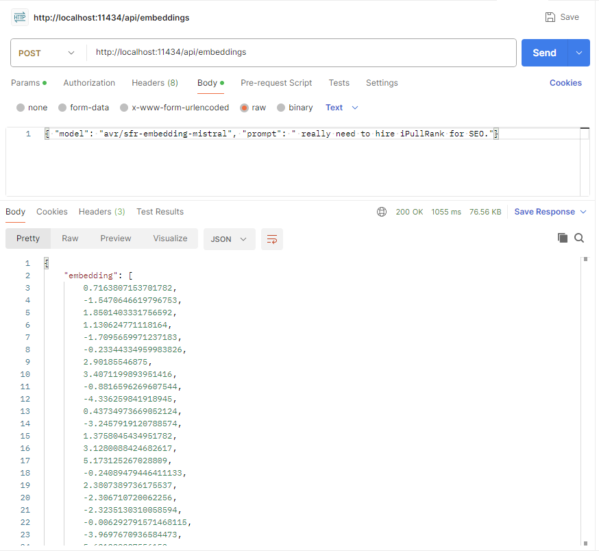
This is all quite inexpensive, but you could also set up an embedding server locally via ollama and generate your embeddings for free using one of the open source pretrained models. For example, if you wanted to use the highly-rated SFR-embedding-mistral embeddings model in the same way, follow these steps:
- Download, install, and start ollama
- Confirm that it’s running by going to http://localhost:11434
- At the command line download and run the model with this command: ollama run avr/
sfr-embedding-mistral. To verify things are working properly you can run a query in Postman or with cURL.
- Once you’ve confirmed it’s running you can use this code as a custom extraction for generating the embeddings.
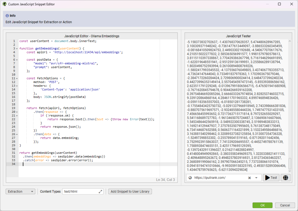
Here’s the code:
const userContent = document.body.innerText;

function getEmbeddings(userContent) {
    const apiUrl = 'http://localhost:11434/api/embeddings';

    const postData = {
        "model": "avr/sfr-embedding-mistral",
        "prompt": userContent,
    };

    const fetchOptions = {
        method: 'POST',
        headers: {
            'Content-Type': 'application/json'
        },
        body: JSON.stringify(postData)
    };

    return fetch(apiUrl, fetchOptions)
        .then(response => {
            if (!response.ok) {
                return response.text().then(text => {throw new Error(text)});
            }
            return response.json();
        })
        .then(data => {
            return data.embedding;
        });
}

return getEmbeddings(userContent)
  .then(embeddings => seoSpider.data(embeddings))
  .catch(error => seoSpider.error(error));
Depending on the specs of your machine, ollama may slow down your crawl too much to use it for generating embeddings. It may timeout before the data is returned. Make sure to test it on a few URLs before you let your crawl go.
Preparing Your Embeddings for Analysis
Before we get into use cases, you need to know how to prepare the data for analysis. Embeddings are stored in SFSS as comma-separated strings, but embeddings are numerical and need to be converted back into floats to be used for analysis. I prefer to export the XLSX file rather than a CSV because too many tools have done me dirty when it comes to formatting. I don’t want any potential formatting issues to damage my hard-won data. However, my testing has shown that CSVs can work just fine here too.
Nevertheless, the conversion is simple with numpy. Here’s a function to make it happen after you load your file into a dataframe:
def convert_strings_to_float(df, col, new_col_name):
  df = df[df[col].isna() == False]
  df[new_col_name] = df[col].str.split(',')
  df[new_float_col] = df[new_float_col].apply(lambda x: np.float64(x))
  df['EmbeddingLength'] = df[new_float_col].apply(lambda x: x.size)

  return df
Now you have your embeddings in a dataframe and ready to use for analysis.
Indexing Your Vector Embeddings
The first thing we want to do is build an index of the vectors so we can search them for various use cases. For vector searching, we’ll use Google’s SCaNN package. Here’s the code:
def scann_search(dataset:np.ndarray, queries: np.ndarray, n_neighbors = 10, distance_measure = "dot_product", num_leaves = 2000, num_leaves_to_search = 100):
  normalized_dataset = dataset / np.linalg.norm(dataset, axis=1)[:, np.newaxis]

  searcher = scann.scann_ops_pybind.builder(normalized_dataset, n_neighbors, distance_measure).tree(
      num_leaves=num_leaves, num_leaves_to_search=num_leaves_to_search, training_sample_size=250000).score_ah(
      2, anisotropic_quantization_threshold=0.2).reorder(100).build()

  return searcher

def convert_scann_arrays_to_urls(arrays: np.array, df: pd.DataFrame,column):
    results = []
    for arr in arrays:
      results.append(df.iloc[arr.flatten()][column].tolist())
    return results

siteDf = siteDf[siteDf['openAiEmbeddings'].isna() == False]
siteDf['openAiEmbeddingsAsFloats'] = siteDf['openAiEmbeddings'].str.split(',')
siteDf['openAiEmbeddingsAsFloats'] = siteDf['openAiEmbeddingsAsFloats'].apply(lambda x: np.float64(x))
siteDf['EmbeddingLength'] = siteDf['openAiEmbeddingsAsFloats'].apply(lambda x: x.size)

if siteDf['EmbeddingLength'].unique().size == 1:
  d = siteDf['EmbeddingLength'].unique() #Number of dimensions for each value
else:
  print('Dimensionality reduction required to make all arrays the same size.')

dataset = np.vstack(siteDf['openAiEmbeddingsAsFloats'].values)
queries = dataset

siteSearcher = scann_search(dataset, queries)
siteSearcher.serialize(index_directory+'/site_scann_index')
I’m using SCaNN, but you could use another package like Facebook’s FAISS or Spotify’s Annoy.
Note: If you don’t want to do this with Python, you could also push the data to BigQuery and use its engine for vector searches.
Vectorizing your Keyword List
In the vector space model, vectors for queries are compared to vectors for documents to determine what are the most relevant documents for a user’s search. So, for much of your comparative analysis, you will want to vectorize your list of keywords to compare against with nearest neighbor searches and other operations. You can use similar code on a CSV of keywords with their landing pages. We’ll want to maintain the landing pages so we can compare against the pages that are considered the most relevant.
Here is the approach to doing it with OpenAI using an export of keyword data from Semrush:
# Function to get embeddings and flatten them for SCANN
def get_openai_embeddings(keyword):
    response = openai.embeddings.create(
        input=keyword,
        model="text-embedding-3-small"  # Make sure to use the same embeddings as Screaming Frog
    )
    # Extract and flatten the embedding
    embedding_vector = response.data[0].embedding
    return np.array(embedding_vector).flatten()

semrushFile = '<a data-ail="17504" target="_blank"  href="https://ipullrank.com/about-ipullrank" title="Ipullrank">ipullrank</a>.com-organic.Positions-us-20220415-2024-05-05T16_03_31Z.csv'
keywordDf = read_file(semrushFile, 'CSV')
display(keywordDf)

# Loop through the DataFrame and get embeddings for each keyword
embeddings = []
for keyword in keywordDf['Keyword']:
    embeddings.append(get_openai_embeddings(keyword))

keywordDf['embeddings'] = embeddings

# Create a temporary DataFrame for Excel output with embeddings converted to strings
tempDf = keywordDf.copy()
tempDf['embeddings'] = tempDf['embeddings'].apply(lambda x: str(x))
tempDf.to_excel('semrush-embeddings.xlsx', index=False) # Save with embeddings as strings

# Display the updated DataFrame
print(keywordDf.head())
If you’re using Google’s embeddings they make a specific distinction between document and query embeddings. So, the code we used earlier will require the “RETRIEVAL_QUERY” task type to be specified. The only change that we make is calling the embed_text() function with the task variable set to RETRIEVAL_QUERY.
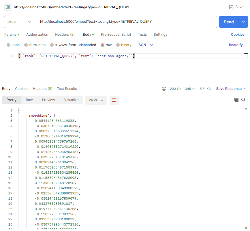
Here’s the adjustment to the code to make that happen:
# Loop through the DataFrame and get embeddings for each keyword
embeddings = []
for keyword in keywordDf['Keyword']:
    <strong>embeddings.append(embed_text(keyword,”RETRIEVAL_QUERY”)
</strong>
Now let’s create a SCaNN index of the keyword list:
embeddings_matrix = np.vstack(keywordDf['embeddings'])

keywordSearcher = scann.scann_ops_pybind.builder(embeddings_matrix, 10, "dot_product").tree(
    num_leaves=200, num_leaves_to_search=100, training_sample_size=250000
).score_ah(2, anisotropic_quantization_threshold=0.2).reorder(100).build()
In case you’re wondering, you should not compare embeddings from different sources because they are not the same length nor are they composed by the same language model. Be consistent with the embeddings model that you use across your analysis.
SEO Use Cases for Vectorized Crawls
Ok, now we can unlock some new capabilities that can enhance the level of analysis we can do. Typically, machine learning engineers use embeddings to do a variety of things, including:
- Clustering – Clustering is the process of grouping a set of objects in such a way that objects in the same group (called a cluster) are more similar to each other than to those in other groups.
- Classification – Classification involves assigning categories to objects based on input features, using trained models to predict the category for new, unseen data. I’m not going to cover classification today because that is worth its own post and I want to collect more spam and helpful content data and show you how to build an embeddings based classifier.
- Recommendations – Recommendation systems suggest relevant items to users based on their preferences and past behavior.
- Similarity and Diversity Measurement – This involves assessing how similar or different objects are from each other, often used in systems that need to understand variations or patterns among data points.
- Anomaly Detection – Anomaly detection identifies rare items, events, or observations which raise suspicions by differing significantly from the majority of the data.
- Information Retrieval – Information retrieval is the process of obtaining relevant information from a collection of resources that satisfies the information need from within large datasets.
- Machine Translation – Machine translation automatically translates text from one language to another, using complex models to understand and convert languages.
- Text Generation – Text generation is the process of automatically producing text, often mimicking human-like writing, using various algorithms and statistical techniques.
This new SF feature unlocks your ability to apply these techniques to drive deep insights for SEO.
Keyword Mapping
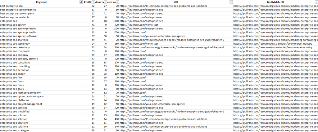
The keyword-to-keyword and keyword-to-page relationships are the most important aspects we can directly impact as content creators and SEOs. Optimizing pages to improve their keyword targeting through copy adjustments and linking strategies is best reinforced through a determination of what page owns what keywords. In some cases, due to the array of ranking factors, you’ll find that what ranks for the keyword is not the best page on your site. To remedy that at scale, you can loop through your keyword vector embeddings and perform nearest neighbor searches on your document SCaNN index. Wherever the highest ranking URL does not match the current landing page, that’s a linking opportunity for optimization.
To do that we perform the search, add the URL to the dataframe and an indication of whether it’s a match. Very quickly we have an understanding of how where we need to improve our keyword targeting.
queries = np.vstack(keywordDf['embeddings'].values) #Stacking all individual embeddings vertically into matrix

kwSearcher = scann_search(dataset, queries) # dataset is the same as before
nearest_neighbors = kwSearcher.search_batched(queries, final_num_neighbors=1)
matched_urls = convert_scann_arrays_to_urls(nearest_neighbors, siteDf, 'Address')

keywordDf['BestMatchURL'] = convert_scann_arrays_to_urls(neighbors, siteDf, 'Address')
keywordDf['BestMatchURL'] = keywordDf['BestMatchURL'].apply(lambda x: x[:1][0])

display(keywordDf)
When we run this, the data tells me that our guide to enterprise SEO is considered more relevant for enterprise SEO queries than our enterprise SEO landing page. Granted, our enterprise SEO page performs better, but looks like we need to optimize our content a bit better if we want the enterprise SEO landing page to rank better.
Keyword Relevance Calculations
The measure of relevance is the function of distance between embeddings. That is calculated in several ways: euclidean distance, dot product, and my preference, cosine similarity. I prefer it because of its simplicity and the ease of converting it into a score between 0 and 100. With the keyword and URL embeddings we can compare the mapped keyword to the URL to determine how relevant it is. You could also crawl competitor pages with SFSS and do the same. The comparison is simple. Find the embeddings for the URL and the keyword in their respective dataframes and perform cosine similarity.
# Function to normalize embeddings
def normalize_embeddings(embeddings):
    norms = np.linalg.norm(embeddings, axis=1, keepdims=True)
    return (embeddings / norms).tolist()  # Normalize and convert to list

# Normalize the embeddings and convert them to lists for DataFrame storage
keywordDf['NormalizedEmbeddings'] = normalize_embeddings(np.vstack(keywordDf['embeddings'].values))
siteDf['NormalizedEmbeddings'] = normalize_embeddings(np.vstack(siteDf['OpenAI Embeddings 1ConvertedFloats'].values))

# Function to calculate cosine similarity
def cosine_similarity(embedding1, embedding2):
    return np.dot(embedding1, embedding2)

# Initialize a list to store cosine similarity results
cosine_similarities = []
relevance_values = []

# Loop through each keyword to calculate cosine similarity with its corresponding URL in siteDf
for index, row in keywordDf.iterrows():
    keyword_url = row['URL']
    keyword_embedding = row['NormalizedEmbeddings']  # This is now a list

    # Find the corresponding URL in siteDf
    if keyword_url in siteDf['Address'].values:
        # Get the embedding for the matching URL, which is also stored as a list
        url_embedding = siteDf.loc[siteDf['Address'] == keyword_url, 'NormalizedEmbeddings'].iloc[0]
        # Convert list to numpy array for calculation
        similarity = cosine_similarity(np.array(keyword_embedding), np.array(url_embedding))
        relevance = similarity * 100
    else:
        similarity = None  # Set similarity to None if no matching URL is found
        relevance = None

    cosine_similarities.append(similarity)
    relevance_values.append(relevance)

# Store the cosine similarities in the keywordDf
keywordDf['CosineSimilarity'] = cosine_similarities
keywordDf['Relevance'] = relevance_values


# Display or use the updated DataFrame
print(keywordDf[['Keyword', 'URL', 'CosineSimilarity','Relevance']])

keywordDf.to_excel('keyword-relevance.xlsx')
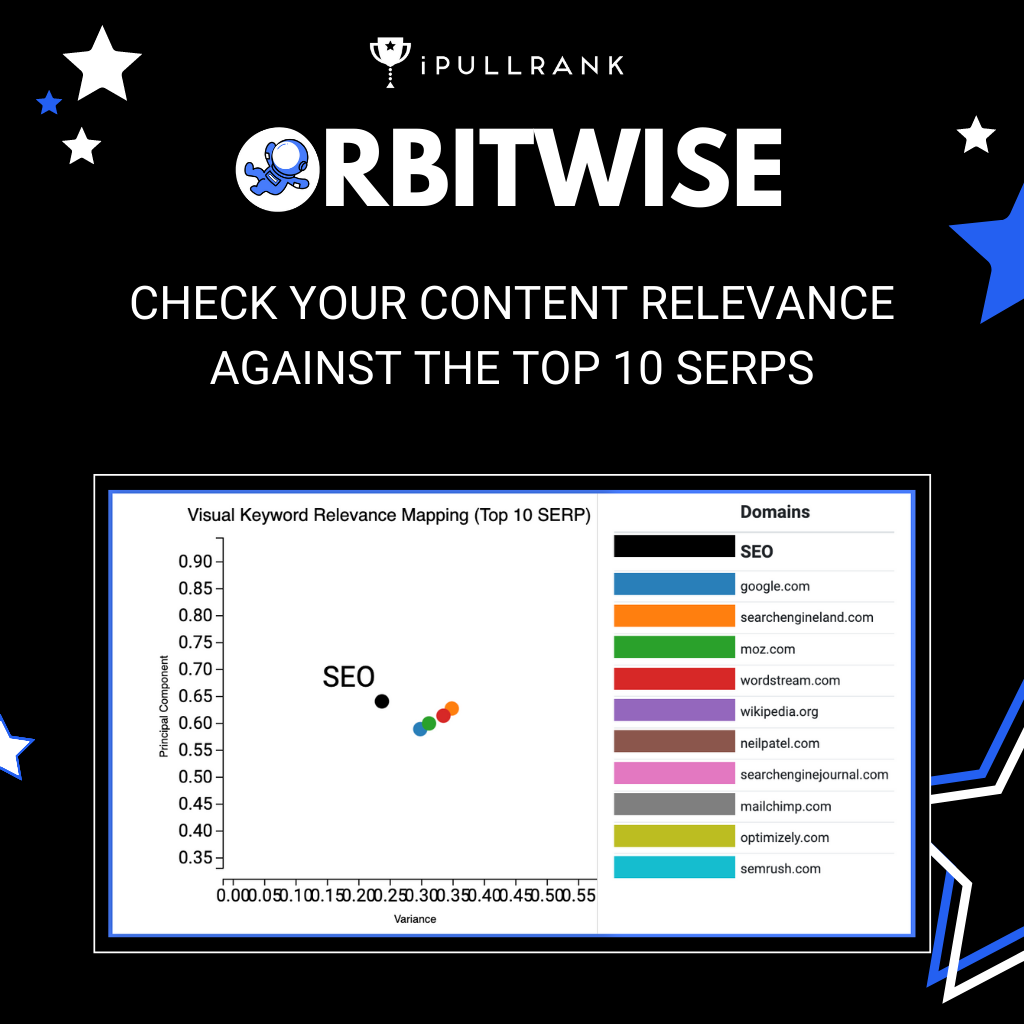
This is what our tool Orbitwise does.
What you’re seeing here is an indication of low middling relevance for these keywords versus these landing pages.

Internal Linking and Redirect Mapping
Link relevance is about parity and the higher the relationship between the source and target URLs, the more valuable the link.
When Overstock was migrating to bedbathandbeyond.com, I talked about how they could map the redirects as scale using nearest neighbor searches. This same concept can be applied to identifying where to build internal links.
As we have mapped our keywords to landing pages, we now have an understanding of the best pages to own which keywords. Such analysis is especially useful when dealing with millions of pages versus millions of keywords. Assuming we want to build 10 links from different pages across the site, we can determine internal link sources for a given page by using keyword searches on the document index or we can do it by doing document searches on the document index.
The code is the same as what we did for keyword mapping, we just want more results. Let’s search for 10 neighbors this time.
# Search siteDf for keywords, return 10 neighbors per keyword

queries = np.vstack(keywordDf['embeddings'].values) #Stacking all individual embeddings vertically into matrix

kwSearcher = scann_search(dataset, queries) # dataset is the same as before
neighbors, distances = siteSearcher.search_batched(queries, leaves_to_search = 150)

nearest_neighbors = kwSearcher.search_batched(queries, final_num_neighbors=5)

matched_urls = convert_scann_arrays_to_urls(nearest_neighbors, siteDf, 'Address')

keywordDf['InternalLinkSuggestions'] = convert_scann_arrays_to_urls(neighbors, siteDf, 'Address')
keywordDf['InternalLinkSuggestions'] = keywordDf['InternalLinkSuggestions'].apply(lambda x: x[1:])
display(keywordDf)

# Create a temporary DataFrame for Excel output with embeddings converted to strings
tempDf = keywordDf.copy()
tempDf['embeddings'] = tempDf['embeddings'].apply(lambda x: str(x))
tempDf.to_excel('keyword-internal-link-mapping.xlsx', index=False) # Save with embeddings as strings
For the document version, we select the document embedding and use it to perform the search on the document index.
queries = dataset

siteSearcher = scann_search(dataset, queries)

neighbors, distances = siteSearcher.search_batched(queries, leaves_to_search = 150)

nearest_neighbors = siteSearcher.search_batched(queries, final_num_neighbors=10)

matched_urls = convert_scann_arrays_to_urls(nearest_neighbors, siteDf, 'Address')

siteDf['PageToPageLinkMapping'] = convert_scann_arrays_to_urls(neighbors, siteDf, 'Address')
siteDf['PageToPageLinkMapping'] = siteDf['PageToPageLinkMapping'].apply(lambda x: x[2:])
display(siteDf)
siteDf.to_excel('page-to-page-link-mapping.xlsx')
Here are the results for our Enterprise SEO page based on the page to page calculations.
['https://ipullrank.com/resources/guides-ebooks/modern-enterprise-seo-guide/chapter-1', 'https://ipullrank.com/', 'https://ipullrank.com/seo-for-the-procurement-professional', 'https://ipullrank.com/services/technical-seo', 'https://ipullrank.com/services', 'https://ipullrank.com/author/andrew-mcdermott/page/3', 'https://ipullrank.com/resources/guides-ebooks/modern-enterprise-seo-guide', 'https://ipullrank.com/11-common-enterprise-seo-problems-and-solutions']For redirect mapping, you’d crawl the old site and the new site to generate embeddings for both. Then search the target site’s index with embeddings to the target site with top k set to 1. Using this data, you can determine the redirect relationships and limit what Google might perceive as soft 404s.
migratingSiteDf = read_file('migrating-site.xlsx', 'Excel')
migratingSiteDf = migratingSiteDf[migratingSiteDf['OpenAIEmbeddings'].isna() == False]
migratingSiteDf = migratingSiteDf[~migratingSiteDf['OpenAIEmbeddings'].str.contains('error')]
migratingSiteDf['OpenAIEmbeddingsFloats'] = migratingSiteDf['OpenAIEmbeddings'].str.split(',')

migratingSiteDf['OpenAIEmbeddingsFloats'] = migratingSiteDf['OpenAIEmbeddingsFloats'].apply(lambda x: np.array(x, dtype = float))

queries = np.vstack(migratingSiteDf['OpenAIEmbeddingsFloats'].values) #Stacking all individual embeddings vertically into matrix

migrationSearcher = scann_search(dataset, queries) # dataset is the same as before
neighbors, distances = migrationSearcher.search_batched(queries, leaves_to_search = 150)

nearest_neighbors = migrationSearcher.search_batched(queries, final_num_neighbors=1)

migratingSiteDf['MigrationTargetSuggestions'] = convert_scann_arrays_to_urls(neighbors, siteDf, 'Address')
migratingSiteDf['MigrationTargetSuggestions'] = migratingSiteDf['MigrationTargetSuggestions'].apply(lambda x: x[:1][0])

display(migratingSiteDf)
migratingSiteDf.to_excel('migration-recommendations.xlsx')
Link Building Target Identification
This is another story for another day, but I do not believe the volume approach for link building works anymore. On the back of the advancements in natural language processing, Google is better at understanding and modeling relevance parity between the source and target of links. Links built from sources that are completely irrelevant to the subject matter are invalidated in modern PageRank calculations. My hypothesis is that this is an aspect of how SpamBrain works.
To that end, we can vectorize a list of pages we are considering for link building and compare them against the target page using cosine similarity to determine how relevant the page source page of the link is.
For this process, we’d:
- Identify a series of link targets using a tool like Ahrefs, Semrush, Pitchbox, or Respona
- Crawl those pages with Screaming Frog to collect their embeddings.
- Compare them against the embeddings for your site to get the cosine similarity.
That yields a table that looks like the one below. When I sort ascending, that lets me know all the URLs that are not good fits for me to get links from. When we look at the scores, if they are not a 0.6 or higher, they are not relevant enough to build links from.

Here’s the code to make it happen:
import pandas as pd
import numpy as np
from scipy.spatial.distance import cdist

# Load the DataFrame
linkProspectsDf = pd.read_excel('link-prospects.xlsx')
linkProspectsDf = linkProspectsDf[linkProspectsDf['OpenAI Embeddings Long Inputs 1'].notna()]
linkProspectsDf = linkProspectsDf[~linkProspectsDf['OpenAI Embeddings Long Inputs 1'].str.contains('error|TypeError', regex=True)]

# Convert the string of numbers into a list of floats
def convert_embeddings(embedding_str):
    try:
        # Split the string into a list of strings, then convert each to float
        return np.array([float(num) for num in embedding_str.split(',')])
    except ValueError:
        # Return None or np.nan in case of conversion failure, which should be handled or filtered later
        return np.nan

linkProspectsDf['OpenAIEmbeddingsFloats'] = linkProspectsDf['OpenAI Embeddings Long Inputs 1'].apply(convert_embeddings)

# Remove rows where embeddings conversion failed (if any)
linkProspectsDf.dropna(subset=['OpenAIEmbeddingsFloats'], inplace=True)

# Normalize the embeddings
linkProspectsDf['normalized_embeddings'] = linkProspectsDf['OpenAIEmbeddingsFloats'].apply(lambda x: x / np.linalg.norm(x))
siteDf['normalized_embeddings'] = siteDf[new_float_col].apply(lambda x: x / np.linalg.norm(x))

# Specific URL to search for
specific_url = 'https://ipullrank.com/enterprise-seo'  # Change this to your specific URL

# Retrieve the normalized embedding for the specific URL
specific_embedding = siteDf[siteDf['Address'] == specific_url]['normalized_embeddings'].values[0]

# Prepare the embeddings array from the second dataframe
embeddings2 = np.stack(linkProspectsDf['normalized_embeddings'].values)

# Calculate cosine similarity
cosine_similarity_scores = 1 - cdist([specific_embedding], embeddings2, 'cosine')[0]

# Create a dataframe to store the results
results = pd.DataFrame({
    'Search Address': specific_url,
    'Target Address': linkProspectsDf['Address'],
    'Cosine Similarity Score': cosine_similarity_scores
})

# Optionally, sort the results by scores
results = results.sort_values(by='Cosine Similarity Score', ascending=False)
results.to_excel('link-prospect-relevance.xlsx')
display(results)
Clustering Content
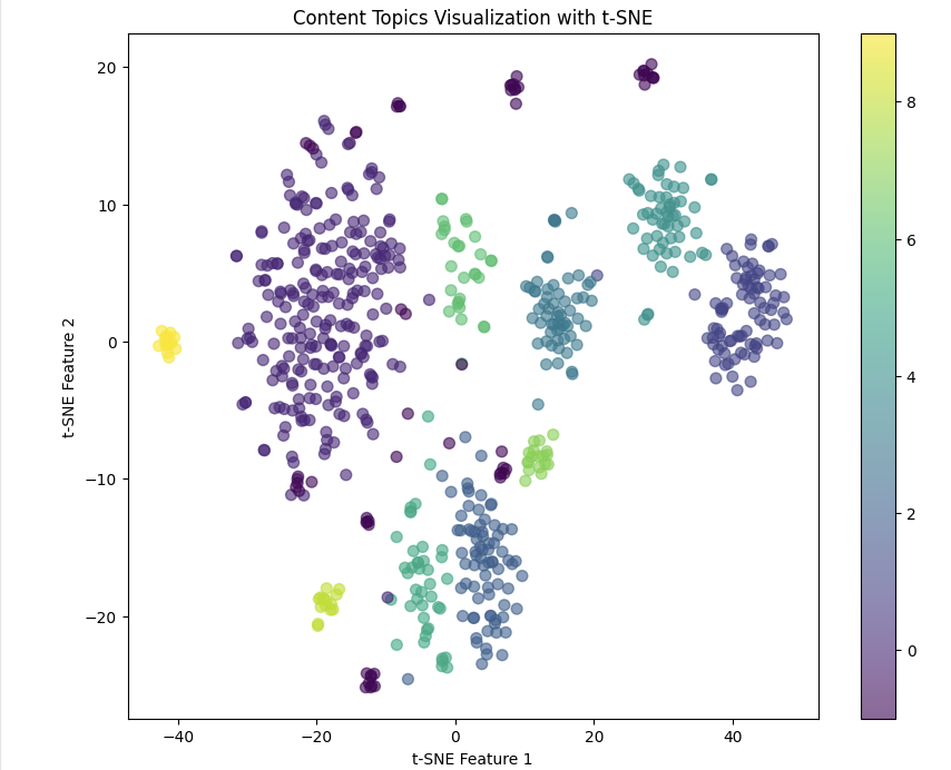
Clustering the content can help us form topical clusters and also identify anomalies where the content is not relevant to any other content on the site. As sites grow larger, it becomes more difficult to manage how often the same topics are covered. Using BERTopic with our embeddings we can build and visualize a topical map of our content. When thinking about how you might want to do some content pruning to further reinforce your clusters this is a great approach.
When we run clustering on the embeddings using BERTopic it automatically puts the content into meaningful groups. BERTopic integrates with ChatGPT which allows you to generate human-readable names of the topic that was modeled. This is a vast improvement over other topical modeling approaches that use keywords from the content as representations rather than user-friendly labels.
Once we run our clustering we can visualize them a few different ways. First as a clustered scatter plot:
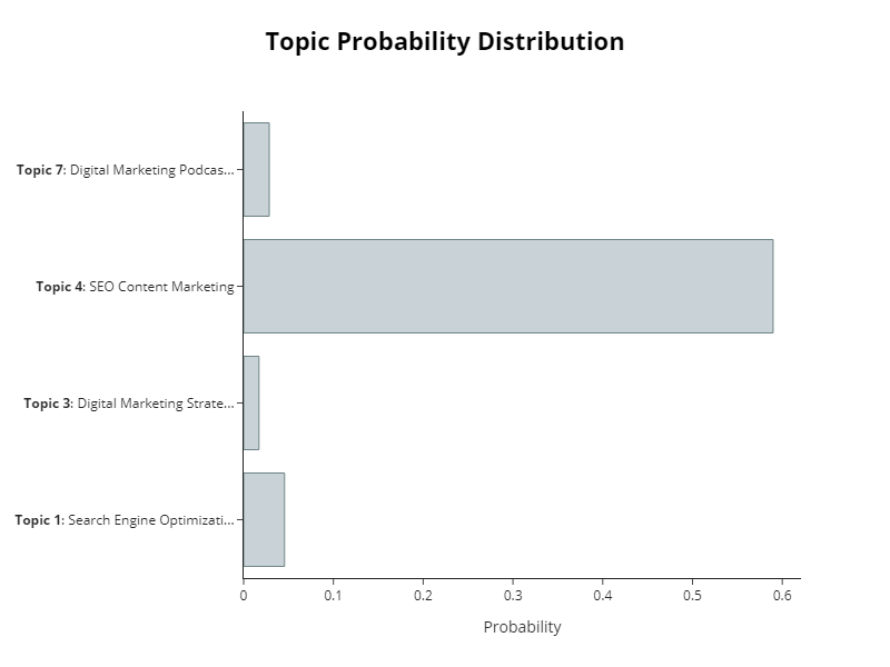
We can also quickly look at the distribution of topics in a bar chart.
And, we can cluster the topics hierarchically.

You can also see how topics are related and not related to each other:
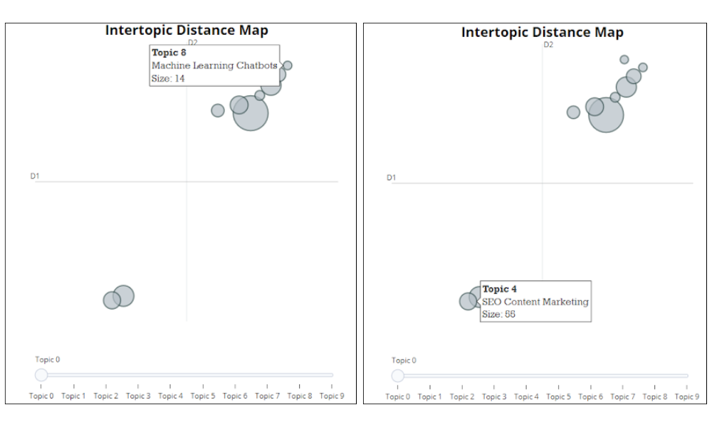
To do this we’ll also need the content itself so we can extract features from it to name the clusters. Capturing the content via SFSS is trivial. The code for the custom function is a one liner:
return seoSpider.data(document.body.innerText);def cluster_and_visualize_content(df, embeddings_col):
print("Starting the <a data-ail="17504" target="_blank" href="https://ipullrank.com/how-topic-modeling-can-improve-your-organic-growth" title="Topic Modeling">topic modeling</a> process for keywords...\n")
# Prepare data
df['Page Content'] = df['Page Content'].astype(str)
keywords = df['Page Content'].tolist()
embeddings = np.vstack(df[embeddings_col].tolist()) # Ensure embeddings are properly shaped
embeddings = normalize(embeddings) # Normalize embeddings for cosine similarity
prompt = """
I have topic that is described by the following keywords: [KEYWORDS]
I am attempting to categorize this topic as part of 2-4 word taxonomy label that encapsulates all the keywords.
Based on the above information, can you give a short taxonomy label of the topic? Just return the taxonomy label itself.
"""
client = openai.OpenAI(api_key=openai.api_key)
representation_model = OpenAI(client, model="gpt-3.5-turbo", prompt=prompt,chat=True)
# Initialize BERTopic
topic_model = BERTopic(representation_model=representation_model,calculate_probabilities=True)
# Fit BERTopic
topics, probabilities = topic_model.fit_transform(keywords, embeddings)
df['topic'] = topics # Adding topic numbers to the DataFrame
# Visualize the topics with t-SNE
print("Reducing dimensions for visualization...")
tsne = TSNE(n_components=2, random_state=42, metric='euclidean')
reduced_embeddings = tsne.fit_transform(embeddings)
plt.figure(figsize=(10, 8))
plt.scatter(reduced_embeddings[:, 0], reduced_embeddings[:, 1], c=topics, cmap='viridis', s=50, alpha=0.6)
plt.colorbar()
plt.title('Content Topics Visualization with t-SNE')
plt.xlabel('t-SNE Feature 1')
plt.ylabel('t-SNE Feature 2')
plt.show()
# Probability distribution visualization
min_probability = 0.01
if any(probabilities[0] > min_probability):
print("Visualizing topic probabilities...")
fig = topic_model.visualize_distribution(probabilities[0], min_probability=min_probability)
fig.show()
else:
print("No topic probabilities above the threshold to visualize.")
# Intertopic distance map
print("Visualizing intertopic distance map...")
fig = topic_model.visualize_topics()
fig.show()
# Hierarchical clustering
print("Visualizing hierarchical clustering...")
fig = topic_model.visualize_hierarchy()
fig.show()
# Extract and name topics
df['topic_name'] = df['topic'].apply(lambda x: topic_model.get_topic(x)[0][0] if topic_model.get_topic(x) else 'No dominant topic')
# Display DataFrame with topic names
display(df)
# Export the DataFrame with topic labels
df.to_excel('content-clusters-bertopic.xlsx', index=False)
pageContentDf = read_file('ipr-content.xlsx', 'Excel')
contentEmbeddingsDf = siteDf.merge(pageContentDf, on='Address', how='inner')
#print(contentEmbeddingsDf)
cluster_and_visualize_content(contentEmbeddingsDf, 'OpenAI Embeddings 1ConvertedFloats')
The Value of a Vector Index of the Web
The democratization of the link graph gave us a series of measures that allowed us to understand the value of websites in the way that Google attributes authority. Granted, those metrics are only approximations of what Google may use, but they have driven the SEO space for nearly two decades.
And, that was enough prior to Google Search’s transition to becoming a heavily machine learning-driven environment. In a hybrid fusion environment, the link graph matters less because Google is taking signals derived from vector embeddings and using them to inform ranking.
Dare I say, the link graph and link indices are less valuable than they were in the past. Whereas all of the above could be native functionality for link indices that make them more valuable for doing SEO moving forward.
Until someone gives us such an index, Screaming Frog has armed us with what we need to catch up to Google.
So, What Are Your Use Cases?
The shortcomings of SEO software has yielded a strong community of Python SEOs. People have been leveraging state of the art technologies to cover the chasm between what SEO software can do and what Google does do.
So, I’m curious, what are your use cases for vector embeddings? How do you anticipate that Screaming Frog’s new feature will help you do your job even better? In the meantime, you can play with all the code I shared in this Colab and contribute your own custom JavaScript snippets at this GitHub. I’ll be back soon with some classification use cases.
Let me know if there’s anything you want me to cook up for you.
Next Steps
Here are 3 ways iPullRank can help you combine SEO and content to earn visibility for your business and drive revenue:
- Schedule a 30-Minute Strategy Session: Share your biggest SEO and content challenges so we can put together a custom discovery deck after looking through your digital presence. No one-size-fits-all solutions, only tailored advice to grow your business. Schedule your consultation session now.
- Mitigate the AI Overviews’ Potential Impact: How prepared is your SEO strategy for Google’s AI Overviews? Get ahead of potential threats and ensure your site remains competitive with our comprehensive AI Overviews Threat Report. Get your AI Overviews report.
- Enhance Your Content Relevancy with Orbitwise: Not sure if your content is mathematically relevant? Use Orbitwise to test and improve your content’s relevancy, ensuring it ranks for your targeted keywords. Test your content relevance today.
Want more? Visit our Resources Page for access to past webinars, exclusive guides, and insightful blogs crafted by our team of experts.





Leave a Comment